Thread by @nassarhuda

The #julialang twitter data network was supposed to be part of this lecture but unfortunately I didn't have enough time -- so here's a thread about it.

How I built it: (1) take the #julialang tweets w >5 likes, (2) get the usernames, (3) find who they follow and build a network.

https://twitter.com/nassarhuda/status/1316809555154698242

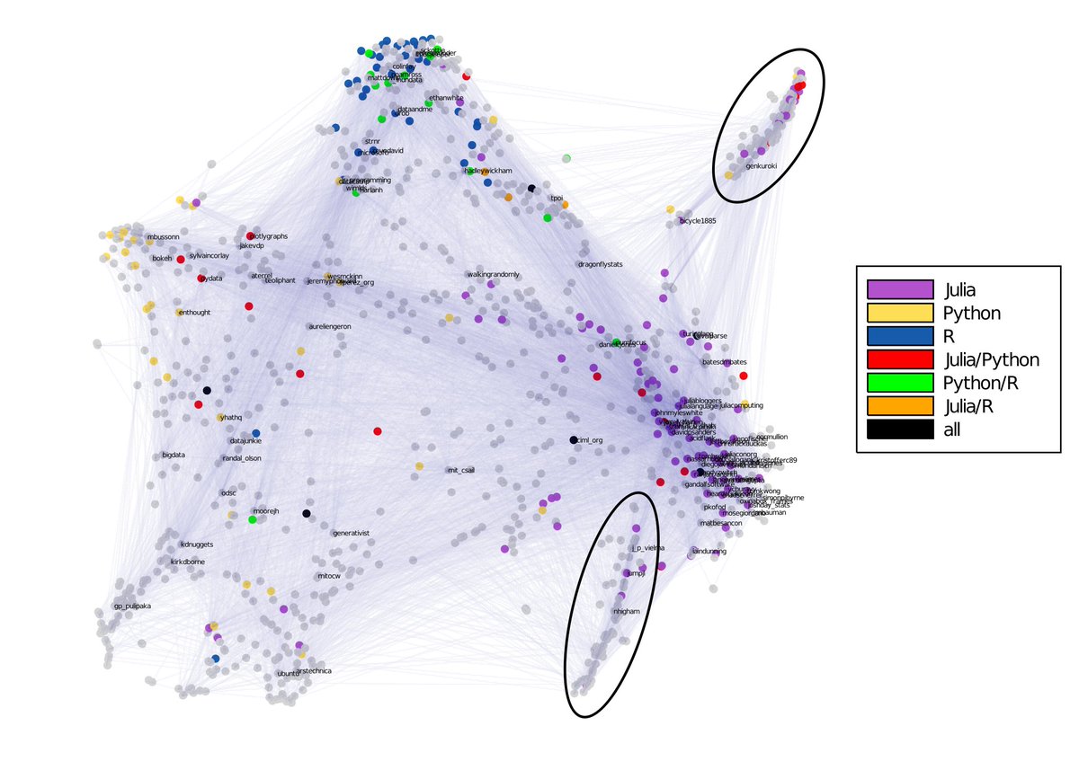
When I first visualized the network, I noticed that there was an apparent separation of some clusters, so the next thing I did is color-coded all the nodes based on whether the words "julia", "python", "rlang"/"rstats" appear in their bios. The resulting figure is pretty amazing!

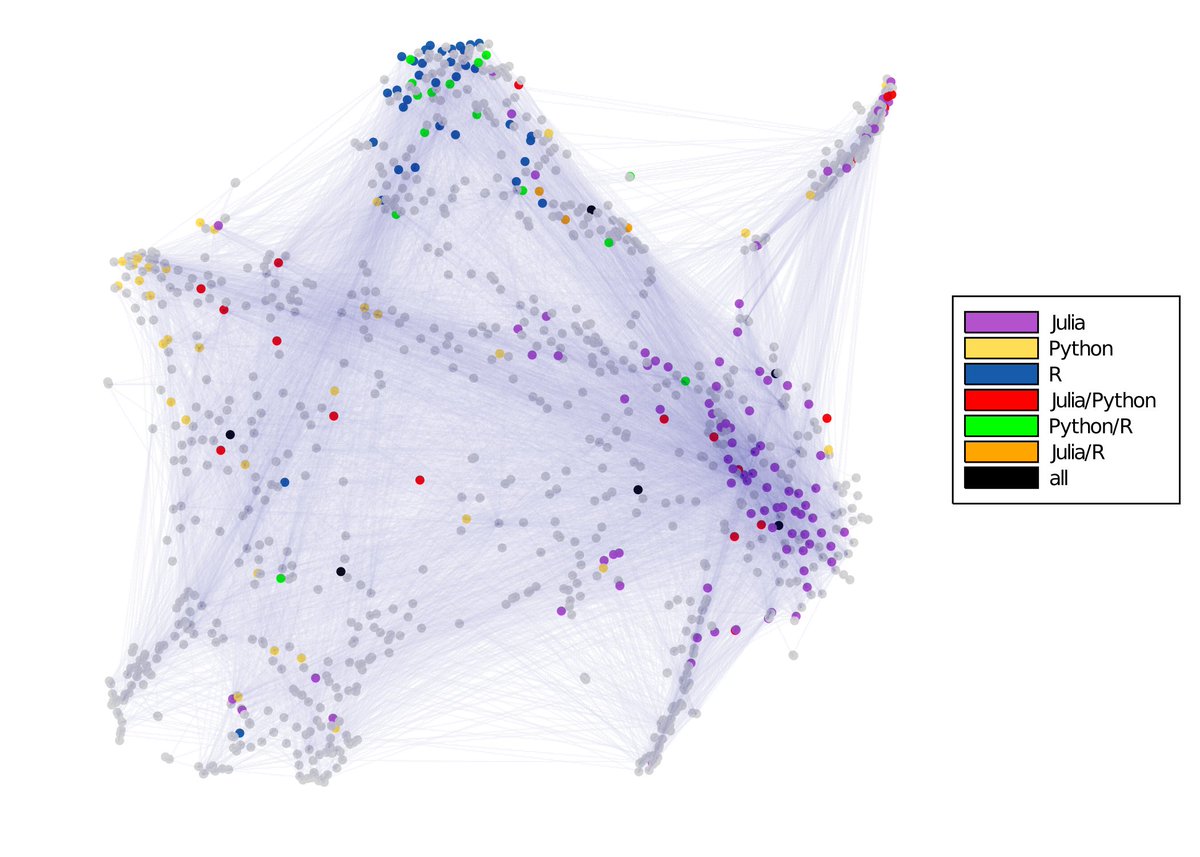
Now if you're like me, you'll probably wonder what's going on with the "two arms" branching out from the julia cluster. So here is an annotated figure w high degree nodes... Fun observation: Everyone I manually inspected in the first group (top in the figure) has a Japanese bio.

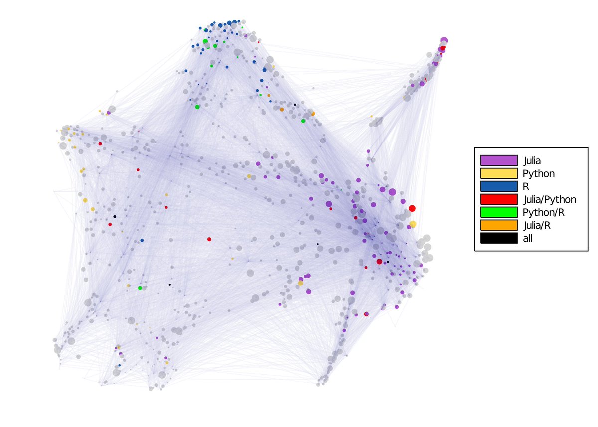
So far, I haven't really given any *numbers*... one thing I was very curious about is to find the clustering coefficients. Here's what I found: the global CC was 0.43, but when I extracted the julia subgraph, the CC jumped to 0.7! Figure: marker size is bigger if local cc >0.5

Here is another local clustering coefficient figure where the marker size is proportional to the local clustering coefficient value.

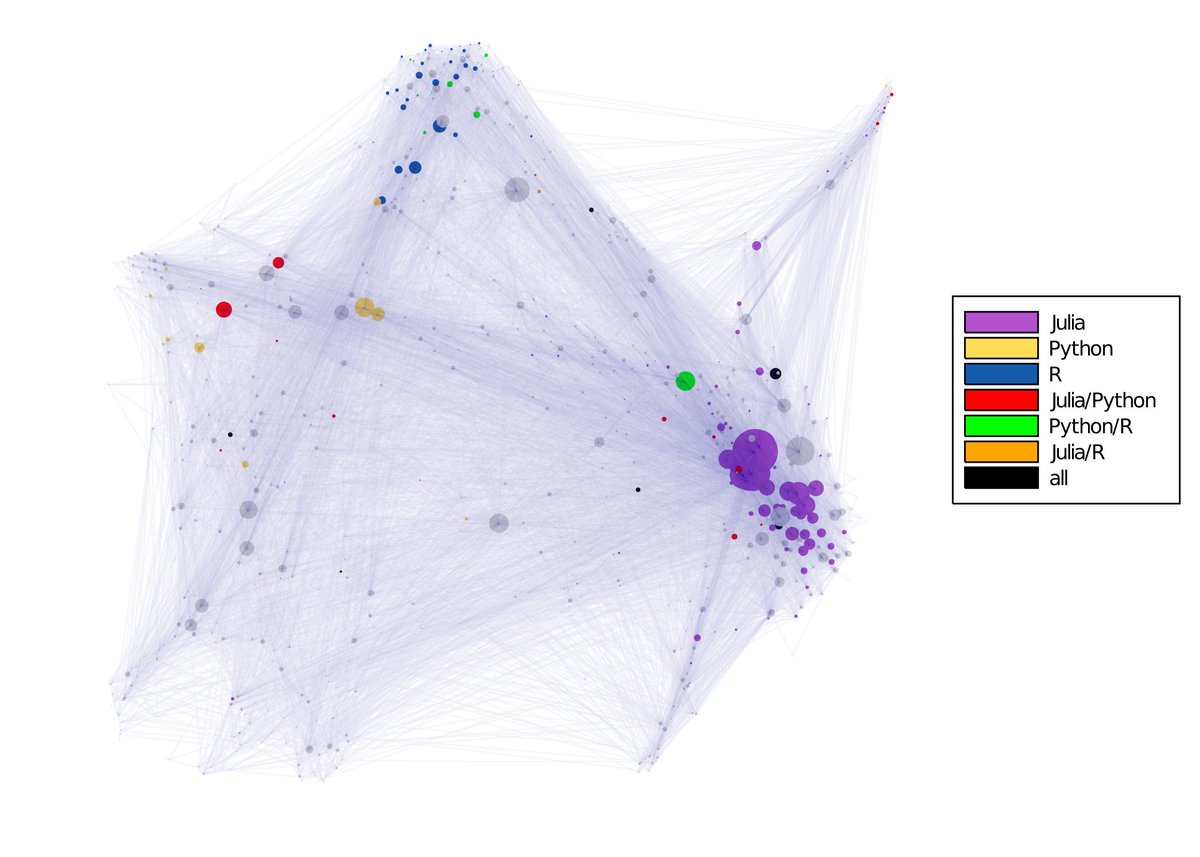
And last but not least... PageRank! Of course, I had to run PageRank on this network. Here is the PageRank visualization with node sizes proportional to the PageRank value... I guess not so surprising, a bunch of the bigger circles were purple circles. 💜

Finally, just some references:
- Code available here: github.com/nassarhuda/MIT…

- Visualization method used: GLANCE -- honestly I was very proud of the visualizations our method, GLANCE, produced (cc: @austinbenson @dgleich). Here's a link to the paper: cs.cornell.edu/~arb/papers/GL…