a 🧵 on M-Estimation and why I think its a valuable tool that epidemiologist should be using more often
M-Estimation is a general approach of defining an estimator as the solution to estimating equations like the following. Importantly, obs are independent and \psi is a known function that doesn't depend on i or n
I think its a great tool for two reasons: (1) the ability to stack estimating equations together, and (2) the sandwich variance
To show (1) consider estimating a MSM with IPW. Here, we have 2 models: the propensity score model and the MSM. M-Estimation means that we can stack these 2 models together for a single procedure and simultaneously estimate both
The ability to stack also relates to (2). The sandwich variance (get it, B is the bread and M is the meat) looks like the following. The advantage of this is that uncertainty can 'flow' through the variance estimation
For IPW-MSM, this means we can stack models together and estimate the sandwich variance. The sandwich variance captures the uncertainty in estimation of the propensity score model, simplifying estimation of the variance
This means we don't have to use the GEE-trick to estimate the variance. The GEE-trick is overly conservative, meaning it represents more uncertainty than necessary
The following is an example I made using my Python library for M-Estimation, delicatessen (yes this is self-promotion). It does all the estimation, derivatives, and matrix algebra for you
github.com/pzivich/Delica…
But you could also recreate everything in R using the geex, which also automates M-Estimation
bsaul.github.io/geex/
Here is a data set I am going to fit both variations of the IPW-MSM on
Here is how I would fit the IPW-MSM using the GEE-trick. The 95% CI is 1.65, 2.52
... and here is the stacked estimating equations and the M-Estimation procedure. The 95% CI is 1.89, 2.28. This is much lower than the GEE version. So the GEE version expresses a much greater uncertainty than necessary
To convince you that M-Estimation is beneficial, here is a short simulation example using a similar mechanism. I ran this for 1000 different data sets
These results demonstrate the over-coverage of the GEE-trick and coverage near expected levels when using M-Estimation. Note the confidence limit difference (CLD), indicative of precision via the difference between UCL and LCL, is almost 1/2 that of GEE!
So M-Estimation is a handy tool, particularly for causal inference and estimation of variances when we need to estimate nuisance models. It also is less computationally intensive than bootstrapping and not overly conservative like the GEE-trick
As here is a good resource for further reading
semanticscholar.org/paper/The-Calc…

• • •

Missing some Tweet in this thread? You can try to force a refresh
 

Keep Current with Pausal Živference

Pausal Živference Profile picture

Stay in touch and get notified when new unrolls are available from this author!

Read all threads

This Thread may be Removed Anytime!

PDF

Twitter may remove this content at anytime! Save it as PDF for later use!

Try unrolling a thread yourself!

how to unroll video
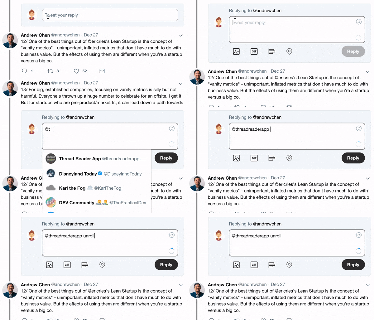
  1. Follow @ThreadReaderApp to mention us!

  2. From a Twitter thread mention us with a keyword "unroll"
@threadreaderapp unroll

Practice here first or read more on our help page!

More from @PausalZ

24 Sep 20
Herd immunity is a far squishier concept then many seem to be describing in their "shielding" or "stratified herd immunity" plans. Here is the formula for herd immunity threshold for a SIR model Image
where \beta is the effective contact rate, N is the number of individuals, and r is the inverse of the duration

The threshold says if are above that level the disease will disappear / we expect no outbreaks of disease. However, that threshold is neither sufficient nor necessary
To show this, let's talk about a perfect vaccine. If you get this vaccine you are perfectly protected from the infection and thus cannot transmit it (everything also applies to imperfect vaccines but it's messier)

Blue circles are vaccinated individuals and red are unvaccinated
Read 15 tweets
20 Sep 20
8: WHEN CAN I IGNORE THE METHODOLOGISTS
Section 8 discusses when standard analytic approaches are fine (aka time-varying confounding isn't as issue for us). Keeping with the occupation theme, it is presented in the context of when employment history can be ignored Image
First we go through the simpler case of point-exposures (ie only treatment assignment at baseline matters). Note that while we get something similar to the modern definition, I don't think the differentiation from colliders is quite there yet (in the language) ImageImage
Generalization of the point-exposure definition of confounding to time-varying exposures isn't direct Image
Read 13 tweets
19 Sep 20
7: MORE ASSUMPTIONS
Section 7 adds some additional a priori assumptions that can allow us to estimate in the context where we don't have all necessary confounders.
We have the beautifully named: A-complete Stage 0 PL-sufficient reduced graph of R CISTG A Image
We start with some rules for reducing graph G_A to a counterpart G_B. Honestly the language in this section isn't clear to me despite reading it several times... ImageImage
I do think the graphs help a bit though. To me it seems we are narrowing the space of the problem. We are going from multiple divisions at t_1 and t_2 to only considering the divisions at t_2 for a single branch. The reduced STG is a single branch ImageImage
Read 6 tweets
15 Sep 20
6: NONPARAM TESTS
Section 6 goes through the sharp null hypothesis (that no effect of exposure on any individual). Note that this is weaker than the null of no _average_ effect in the population Image
Another way of thinking about this is if there is no individual causal effect (ICE) then there must be no average causal effect (ACE). The reverse (no ACE then no ICE) is not guaranteed
Robins provides us with the G-null hypothesis as a means of assessing the sharp null (the g-null is that call causal parameters are 0) ImageImageImage
Read 9 tweets
13 Sep 20
5: ESTIMATION
After a little hiatus, back to discussing Robins 1986 (with a new keyboard)! Robins starts by reminding us (me) that we are assuming the super-population model for inference Image
If we had a infinite n in our study, we could use NPMLE. However, time-varying exposures have a particular large number of possible intervention plans. We probably don't have anywhere near enough obs to consider all the possible plans Image
Instead we use a parametric projection of the time-varying variables. We hope that the parametric projection is sufficiently flexible to approx the true density function (it is why it is best to include as many splines and interaction terms as feasible)
Read 8 tweets
22 Aug 20
4: FORMAL CAUSAL INFERENCE (ATTIRE REQUESTED)
Math on twitter dot com? Should be fine /s
Shorter thread though Image
In Section 4.C we get a quirk of the deterministic results. Essentially within the deterministic system that nature created, the exposure pattern between t_0 and the end of the study has been ‘set’, no matter when outcomes occur. This is used to extend to competing risks Image
Here we get the written version of g-comp from Section 3. There is also the important point that g-comp can be applied to non-causal scenarios. However, when we do this there is less solid of interpretational foundations for the estimate Image
Read 7 tweets

Did Thread Reader help you today?

Support us! We are indie developers!


This site is made by just two indie developers on a laptop doing marketing, support and development! Read more about the story.

Become a Premium Member ($3/month or $30/year) and get exclusive features!

Become Premium

Too expensive? Make a small donation by buying us coffee ($5) or help with server cost ($10)

Donate via Paypal

Thank you for your support!

Follow Us on Twitter!

:(