"The boundary of a boundary is always empty."
A huge amount of (classical) physics, including much of general relativity and electromagnetism, can be deduced directly from this simple mathematical fact.
Yet, on the surface, it doesn't seem to have much to do with physics. (1/10)
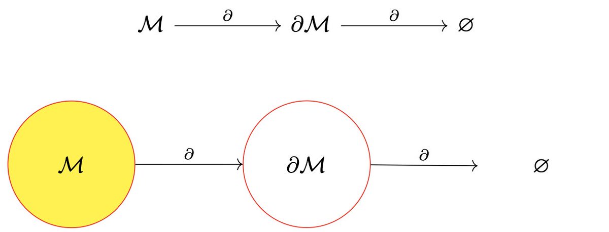
Some spaces (like spheres) don't have boundaries. But, when the boundary exists, it's always one dimension lower (codimension-1). A disc is a 2-dimensional space, but its boundary is a 1-dimensional circle.
But what's the boundary of a circle? Well, it doesn't have one. (2/10)
It turns out that this will always be true, for purely topological reasons: a space may or may not have a boundary, but its boundary never will.
Yet physics is about differential equations, not topology, right? So how can this fact have any relevance to physics? (3/10)
Well, the boundary operator, which maps a space to its boundary space, acts formally very much like a derivative (obeys the product rule, etc.). This is no coincidence: the boundary operator on submanifolds is dual to the exterior derivative operator on differential forms. (4/10)
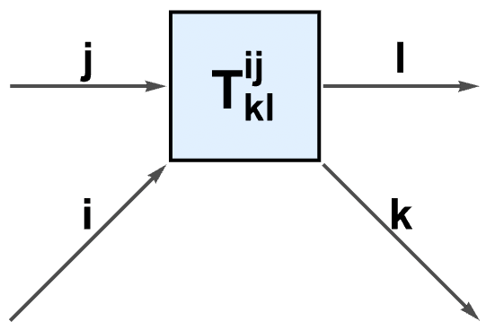
This allows us to translate topological statements about boundaries into analytic statements about exterior derivatives. So our "boundary of a boundary is empty" statement now becomes a statement about symmetries of the covariant derivative operator on certain tensors. (5/10)
When applied to the Riemann tensor and then contracted, it yields the contracted Bianchi identities: the statement that the covariant divergence of the Einstein tensor vanishes. But, in GR, the Einstein tensor is equal to the stress-energy tensor (times a constant). (6/10)
So the covariant divergence of stress-energy vanishes - in physical terms, this means that energy and momentum are always conserved in relativity!
If instead we apply the Bianchi identities to the electromagnetic field tensor, we obtain the (homogeneous) Maxwell equations. (7/10)
These encompass both Gauss' law for magnetism and the Maxwell-Faraday law of induction.
In fact, under the gravitoelectromagnetic formalism, the entirety of general relativity can be represented in this way. Just start by choosing a unit timelike vector field... (8/10)
This field allows us to decompose the Riemann/Weyl tensors into electrogravitic and magnetogravitic tensors (via the Bel decomposition), formally analogous to electric and magnetic field vectors. And, just as for Maxwell, the Bianchi identities give us the dynamical laws. (9/10)
Within this formalism, the full system of Einstein equations emerge as rank-2 tensorial analogs of the rank-1 (vector) Maxwell equations. Yet, somehow, it all goes back to boundaries of boundaries, and their emptiness... (10/10)
• • •
Missing some Tweet in this thread? You can try to
force a refresh
A few people have asked what "fully covariant computation" means, with regards to my last post. I'm currently writing up a big paper about this, but since that will take a while to finish, let me try explaining the basic idea.
Consider, for a moment, general relativity... (1/9)
Often, when we think of solving the Einstein equations, we think of defining initial data on a spacelike hypersurface (a Cauchy surface, or "instantaneous snapshot") and then evolving it forwards in time.
But general covariance means that this is not the only way to do it. (2/9)
Since GR does not ultimately distinguish space and time, we could equally have defined our "initial data" on a timelike hypersurface, and evolved it "sideways" through space, or any mixture of the two (we can even evolve in multiple "time" directions simultaneously). (3/9).
Here's a quick story about comonads, and how they can be used to unify various concepts in functional programming, category theory, rewriting systems and multicomputation. It starts with a practical problem: how to implement better compositional rewriting in Mathematica. (1/11)
First, a brief recap of some basic functional programming/category theory. A “functor” is just a Map in Mathematica: it allows one to apply a function to every element of a data structure (e.g. a list), whilst still preserving the "shape" of that data structure. (2/11)
[The name “functor” here refers to the fact that, if we consider each data structure to be a category, then a Map that doesn't change the "shape" of a structure consequently represents a homomorphism between the respective categories, and hence a functor.] (3/11)
Shock waves, solitons and spacetime singularities: what do sonic booms and water ripples have to do with cosmic censorship and the determinism (or otherwise) of general relativity?
Brace for a brief adventure in hyperbolic partial differential equations (PDEs). (1/20)
PDEs may be broadly classified into three types: elliptic, which are time-independent and where information propagation is instantaneous; parabolic, which are time-dependent and diffusive; and hyperbolic, which are time-dependent and non-diffusive (i.e. wavelike). (2/20)
Hyperbolic PDEs are quite special, and can be analyzed using the method of “characteristics”, in which the PDE is reduced to a family of ordinary differential equations (ODEs), each of which is associated to a path through spacetime called a "characteristic line/curve". (3/20)
[This is part 2 of my series on tensor calculus, differential geometry, etc.]
These blobs are called "tensors", and the "rank" of a tensor represents how many legs it has. Here's a rank-4 tensor with two contravariant indices (inputs) and two covariant indices (outputs). (1/11)
We can build higher-rank tensors out of lower-rank ones by stacking the blobs on top of each other; for instance, here we have assembled a rank-4 tensor out of two rank-2 tensors. As an equation: "M_{j}^{i} N_{l}^{k} = T_{j l}^{i k}". This is called a "tensor product". (2/11)
We can also turn higher-rank tensors into lower-rank ones by connecting wires; for instance, here we have turned a rank-4 tensor into a rank-2 tensor by plugging an output into an input. As an equation: “T_{k i}^{i j} = M_{k}^{j}”. This is called “index contraction”. (3/11)
Lots of pop-sci talks about general relativity and quantum mechanics being “incompatible”, but what does that really mean? And how do quantum field theory, curved spacetime and (effective) quantum gravity fit into that picture? It's a surprisingly interesting story... (1/17)
One of the most important features of quantum mechanics is that it is *linear*: when we add two solutions to the Schrödinger equation together, the result is always another solution to the Schrödinger equation. Physically, this corresponds to the superposition principle. (2/17)
Namely, the linearity of the Schrödinger equation follows from the fact that, if a system can be in one of two possible states, then it can also be in a "superposition" (i.e. a complex linear combination) of those two states - in stark contrast to classical mechanics. (3/17)
[This thread is hopefully(!) the first in a series on tensor calculus, differential geometry and the foundations of general relativity...]
This is a blob. This blob has no inputs and no outputs, so we shall refer to it as a "scalar", and we denote it by an "S". (1/10)
This is a one-legged blob. This blob has one input (denoted "i") and no outputs, so we shall refer to it as a "vector", and we denote it by "V^i" with a superscript. The superscripted (input) index "i" is referred to as a "contravariant" index. (2/10)
This is another one-legged blob. This blob has one output (also denoted "i") and no inputs, so we shall refer to it as a "covector" (or a "one-form"), and we denote it by "V_i" with a subscript. The subscripted (output) index "i" is referred to as a "covariant" index". (3/10)