Post

How to get URL link on X (Twitter) App

On the Twitter thread, click on or icon on the bottom
Click again on or Share Via icon
Click on Copy Link to Tweet
Paste it above and click "Unroll Thread"!
More info at Twitter Help

Peyman Milanfar

@docmilanfar

Mar 29, 2020 • 6 tweets • 3 min read • Read on X

Scrolly

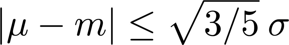
(1/5) One of the most surprising and little-known results in classical statistics is the relationship between the mean, median, and standard deviation. If the distribution has finite variance, then the distance between the median and the mean is bounded by one standard deviation.

(2/5) We assigned this as a HW exercise in a class I taught as a grad student at MIT circa 1991

Coincidentally, it was written up around the same time by C. Mallows in "Another comment on O'Cinneide" The American Statistician, 45-3

Proof is easy using Jensen's inequality twice:

(3/5) If the distribution is unimodal, the bound is even tighter.
epubs.siam.org/doi/10.1137/S0…

(4/5) What about in higher dimensions?

Yes, defining the median appropriately, that works too: median here is the "spatial median": the (unique) point m minimizing the sum of distances E(|x-m|-|x|) to the sample points.

The result appears in this book:
amazon.com/Random-Vectors…

(5/5) Results like this are not just curiosities, but quite useful in practice as they allow estimates of one quantity given the other two in a distribution-free manner. This is important in meta-analyses of studies in biomedical sciences etc

(Open Access) ncbi.nlm.nih.gov/pmc/articles/P…

https://twitter.com/docmilanfar/status/1409368685219770371

https://twitter.com/docmilanfar/status/1409368685219770371

• • •

Missing some Tweet in this thread? You can try to force a refresh

This Thread may be Removed Anytime!

Twitter may remove this content at anytime! Save it as PDF for later use!

More from @docmilanfar

Peyman Milanfar

@docmilanfar

Jan 20

Years ago when my wife and I we were planning to buy a home, my dad stunned me with a quick mental calculation of loan payments.

I asked him how -he said he'd learned the strange formula for compound interest from his father, who was a merchant born in 19th century Iran

1/4

The origins of the formula my dad knew is a mystery, but I know it has been used in the bazaar's of Iran (and elsewhere) for as long as anyone can remember

It has an advantage: it's very easy to compute on an abacus. The exact compounding formula is much more complicated

2/4

I figured out how the two formulae relate: the historical formula is the Taylor series of the exact formula around r=0.

But the crazy thing is that the old Persian formula goes back 100s (maybe 1000s) of years before Taylor's, having been passed down for generations

3/4

Read 4 tweets

Peyman Milanfar

@docmilanfar

Oct 4, 2025

How Kernel Regression is related to Attention Mechanism - a summary in 10 slides.

0/1

1/10

2/10

Read 13 tweets

Peyman Milanfar

@docmilanfar

Aug 22, 2025

Yesterday at the @madebygoogle event we launched "Pro Res Zoom" Pixel 10Pro series. I wanted to share a little more detail, some examples and use cases. The feature enables a combined optical + digital zoom up to 100x magnification. It builds on our optical 5x tele camera.

1/n

Shooting at mags well above 30x requires that the 5x optical capture be adapted and optimized for such conditions, yielding a high quality crop that's fed to our upscaler. The upscaler is a large enough model to understand some semantic context to try & minimize distortions

2/n

Given the distances one might expects to shoot at such high magnification, it's difficult to get every single detail in the scene right. But we always aim to minimize unnatural distortions and stay true to the scene to the greatest extent possible.

3/n

Read 5 tweets

Peyman Milanfar

@docmilanfar

Jul 14, 2025

Receiver Operating Characteristic (ROC) got its name in WWII from Radar, invented to detect enemy aircraft and ships.

I find it much more intuitive than precision/recall. ROC curves show true positive rate vs false positive rate, parametrized by a detection threshold.

1/n

ROC curves show the performance tradeoffs in a binary hypothesis test like this:

H₁: signal present
H₀: signal absent

From a data vector x, we can write ROC directly in terms of x. But typically, some T(x) - a test statistic - is computed, and compared to a threshold γ

2/n

ROC curves derived from general likelihoods are always monotonically increasing

This is easy to see from the definition of Pf and Pd. The slope of the ROC curve is non-negative.

Pro-tip: If you see a ROC curve in a paper or talk that's not so, ask why.

3/n

Read 5 tweets

Peyman Milanfar

@docmilanfar

Apr 30, 2025

The choice of nonlinear activation functions in neural networks can be tricky and important.

That's because iterating (i.e. repeatedly composing) even simple nonlinear functions can lead to unstable, or even chaotic behavior, even with something as simple as a quadratic.

1/n

Some activations are more well-behaved than others. Take ReLU for example:

r(x) = max{0,x}

its iterates are completely benign r⁽ⁿ⁾(x) = r(x), so we don't have to worry.

Most other activations like soft-plus are less benign, but still change gently with composition.

2/n

Soft-plus:

s(x) = log(eˣ + 1)

has a special property: its n-times self-composition is really simple

s⁽ⁿ⁾(x) = log(eˣ + n)

With each iteration, s⁽ⁿ⁾(x) changes gently for all x.

This form is rare -- most activations don't have a nice closed form iterates like this

3/n

Read 7 tweets

Peyman Milanfar

@docmilanfar

Mar 18, 2025

Tweedie's formula is super important in diffusion models & is also one of the cornerstones of empirical Bayes methods.

Given how easy it is to derive, it's surprising how recently it was discovered ('50s). It was published a while later when Tweedie wrote Stein about it

1/n

The MMSE denoiser is known to be the conditional mean f̂(y) = 𝔼(x|y). In this case, we can write the expression for this conditional mean explicitly:

2/n

Note that the normalizing term in the denominator is the marginal density of y.

3/n

Read 8 tweets

Support us! We are indie developers!

This site is made by just two indie developers on a laptop doing marketing, support and development! Read more about the story.

Become a Premium Member ($3/month or $30/year) and get exclusive features!

Become Premium

Don't want to be a Premium member but still want to support us?

Make a small donation by buying us coffee ($5) or help with server cost ($10)

Donate via Paypal

Or Donate anonymously using crypto!

Ethereum

0xfe58350B80634f60Fa6Dc149a72b4DFbc17D341E copy

Bitcoin

3ATGMxNzCUFzxpMCHL5sWSt4DVtS8UqXpi copy

Thank you for your support!

Share this page!

Enter URL or ID to Unroll

Peyman Milanfar

Try unrolling a thread yourself!

More from @docmilanfar

Peyman Milanfar

Peyman Milanfar

Peyman Milanfar

Peyman Milanfar

Peyman Milanfar

Peyman Milanfar

Did Thread Reader help you today?

Don't want to be a Premium member but still want to support us?

Send Email!