
Distinguished Scientist at Google. National Academy of Engineering. Computational Imaging ∩ AI. Posts are personal opinions
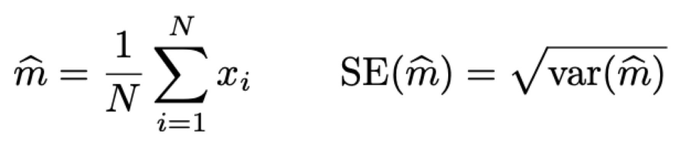 Since m̂ is itself a random variable, we need to quantify the uncertainty around it too: this is what the Standard Error does.
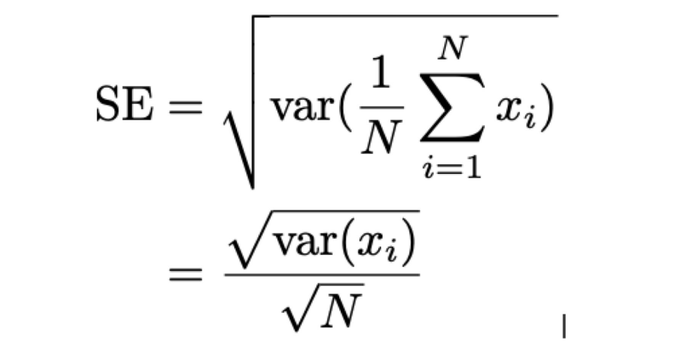
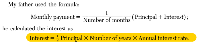 The origins of the formula my dad knew is a mystery, but I know it has been used in the bazaar's of Iran (and elsewhere) for as long as anyone can remember
 1/10
1/10 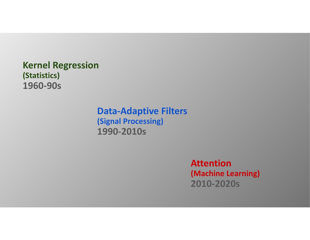


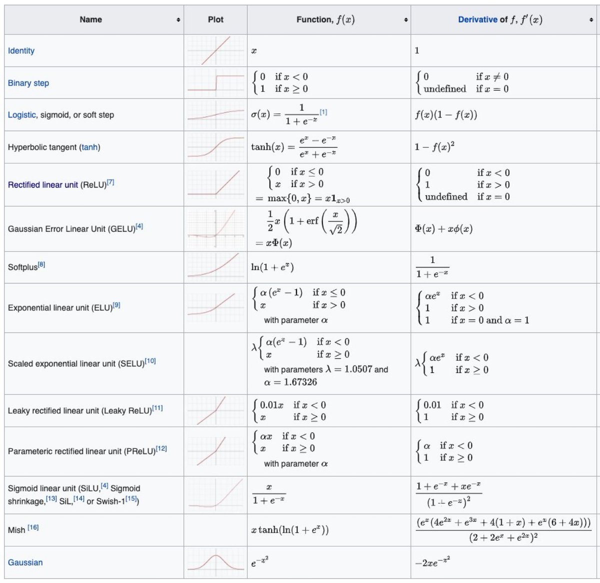 Some activations are more well-behaved than others. Take ReLU for example:
 The MMSE denoiser is known to be the conditional mean f̂(y) = 𝔼(x|y). In this case, we can write the expression for this conditional mean explicitly:
 Images can be thought of as vectors in high-dim. It’s been long hypothesized that images live on low-dim manifolds (hence manifold learning). It’s a reasonable assumption: images of the world are not arbitrary. The low-dim structure arises due to physical constraints & laws
 I once had to explain the Kalman Filter in layperson terms in a legal matter with no maths. No problem - I thought. Yet despite being taught the subject by one of the greats (A.S. Willsky) & having taught the subject myself, I found this very difficult to do.
 The "Silicon Valley Fever Dream" is that data will create knowledge, which will lead to super intelligence, and a bunch of people will get very rich.....
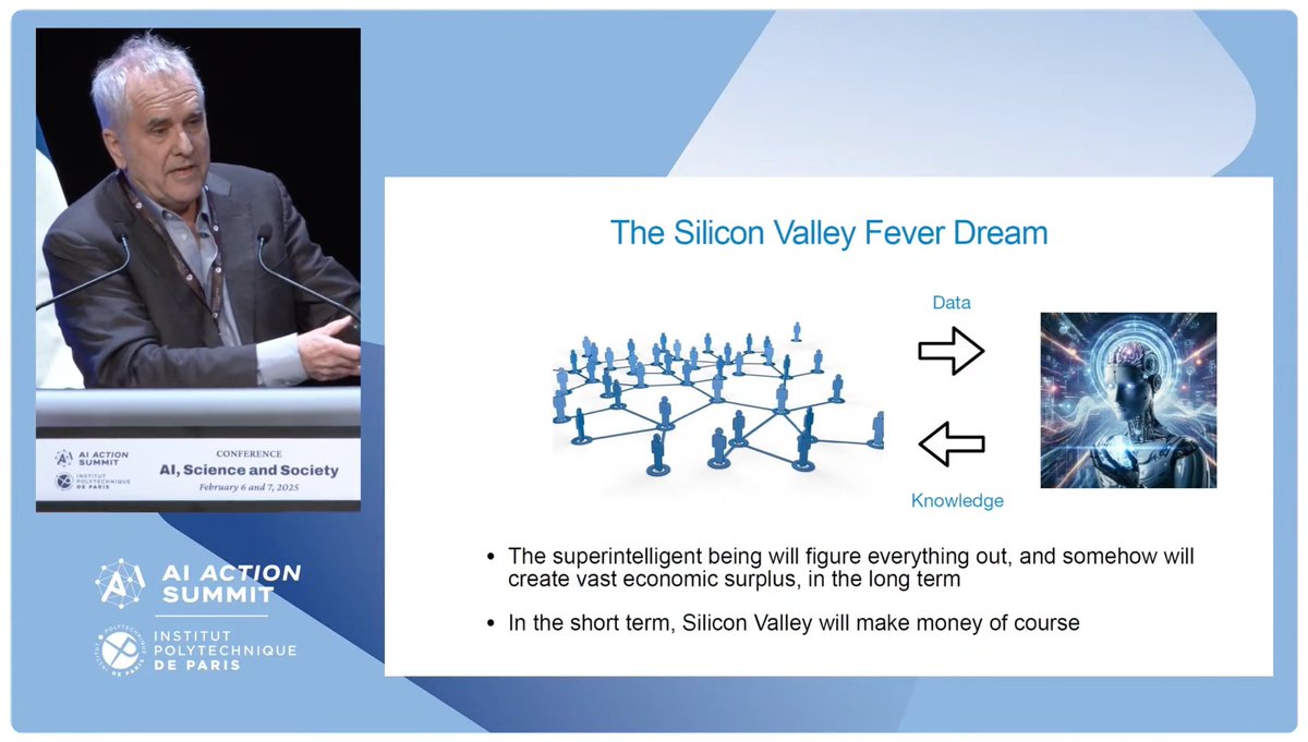
 In the beginning there was Kernel Regression - a powerful and flexible way to fit an implicit function point-wise to samples. The classic KR is based on interpolation kernels that are a function of the position (x) of the samples and not on the values (y) of the samples.
 The origins of the formula my dad knew is a mystery, but I know it has been used in the bazaar's of Iran (and elsewhere) for as long as anyone can remember
 In the beginning there was Kernel Regression - a powerful and flexible way to fit an implicit function point-wise to samples. The classic KR is based on interpolation kernels that are a function of the position (x) of the samples and not on the values (y) of the samples.
 A plot of empirical data can reveal hidden phenomena or scaling. An important and common model is to look for power laws like
 A curve is a collection of tiny segments. Measure each segment & sum. You can go further: make the segments so small they are essentially points, count the red points
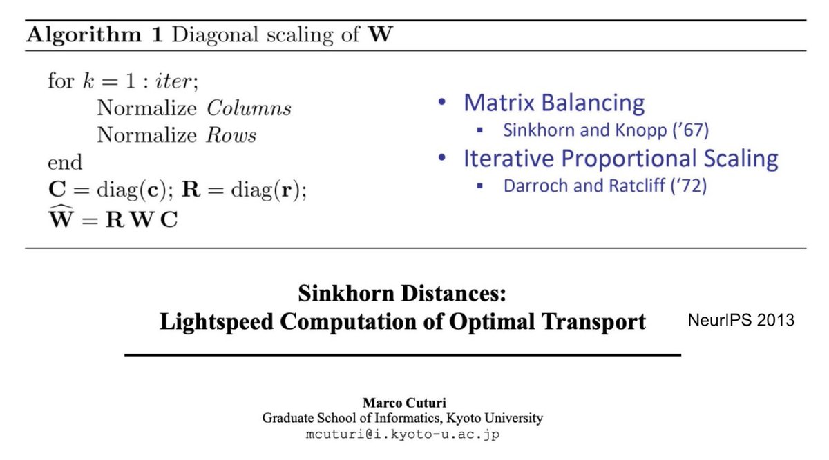
 This is just one instance of how one can “kernelize” an optimization problem. That is, approximate the solution of an optimization problem in just one-step by constructing and applying a kernel once to the input

 If n ≥ p (“under-fitting” or “over-determined" case) the solution is