Thread by @DavidSalazarVir

Trying to get my head around fat-tails by studying @nntaleb's latest technical book. Replicated some plots in #rstats #tidyverse
david-salazar.github.io/2020/04/17/fat…

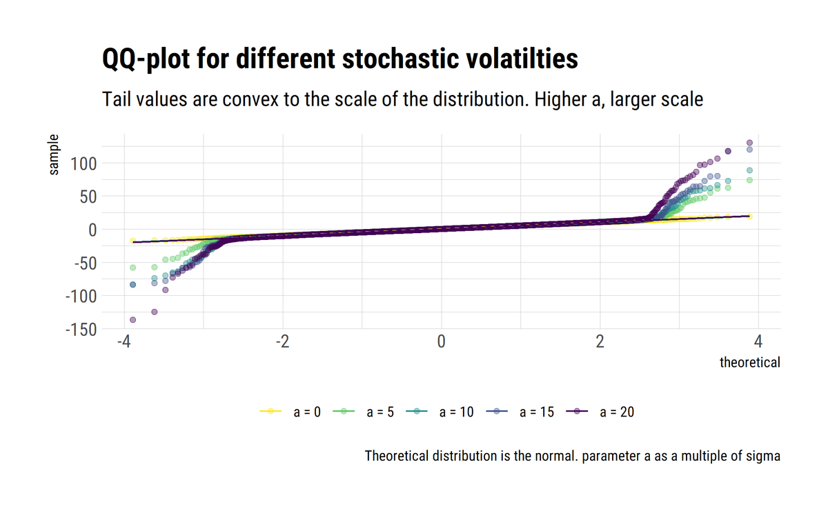
#rstats and @nntaleb's work. By fattening the tails, one learns that the tail events are convex to the scale of the distribution. Thus, the problem compunds: tail events have an increasingly large role, but we cannot estimate their probabilities reliably

david-salazar.github.io/2020/05/09/wha…

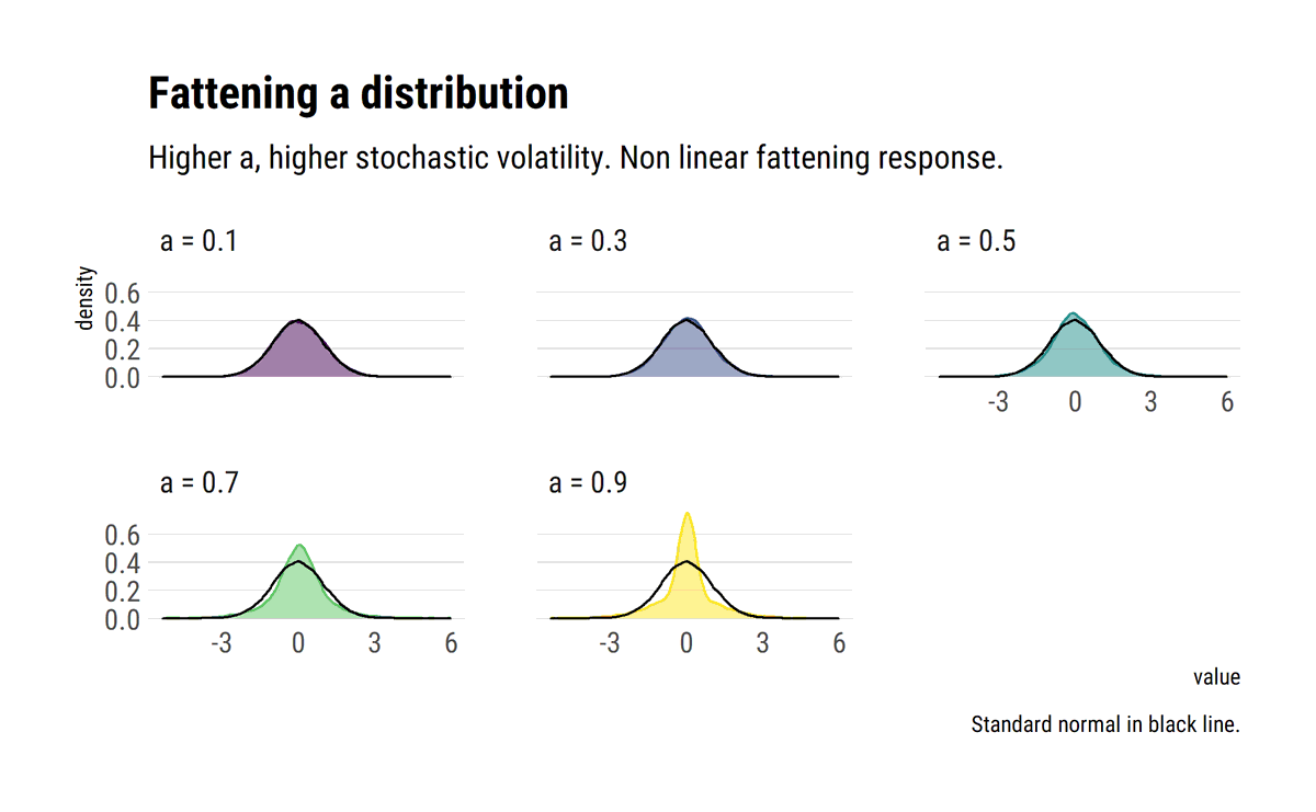
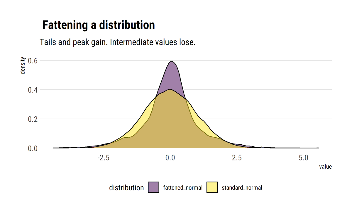
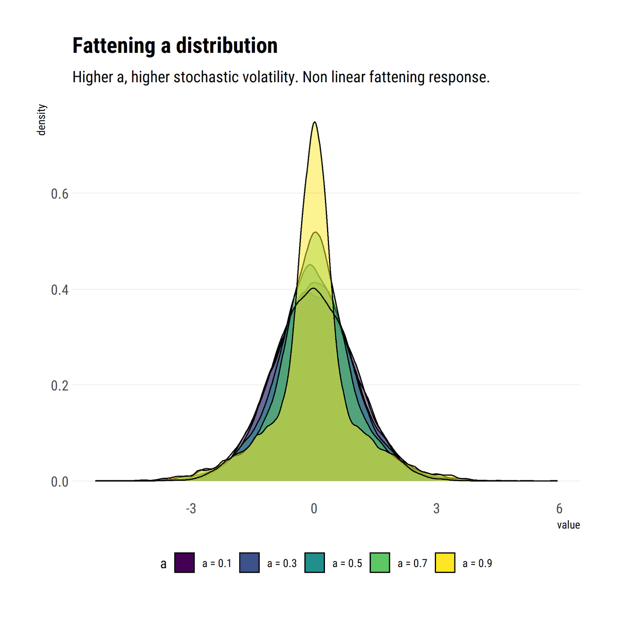
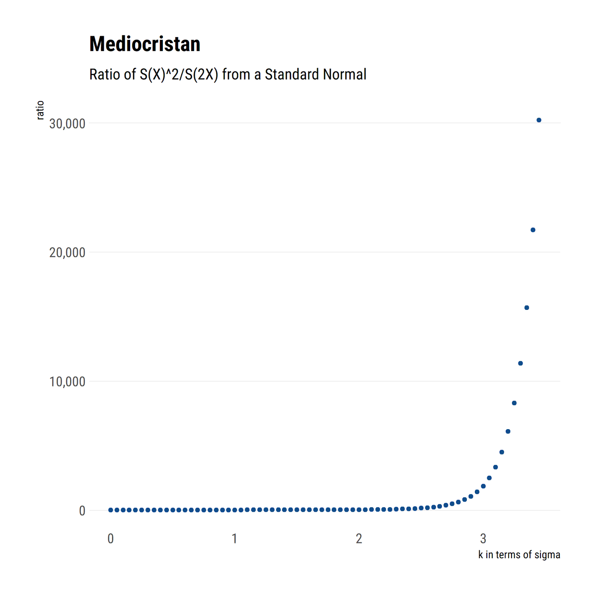
Standard deviation is not intuitive and, outside Mediocristan, the wrong measure of scale. With a simple heuristic to fatten the tails, @nntaleb shows that small deviations wash away the efficiency of SD. MAD is a better measure of scale #rstats

david-salazar.github.io/2020/05/13/sta…

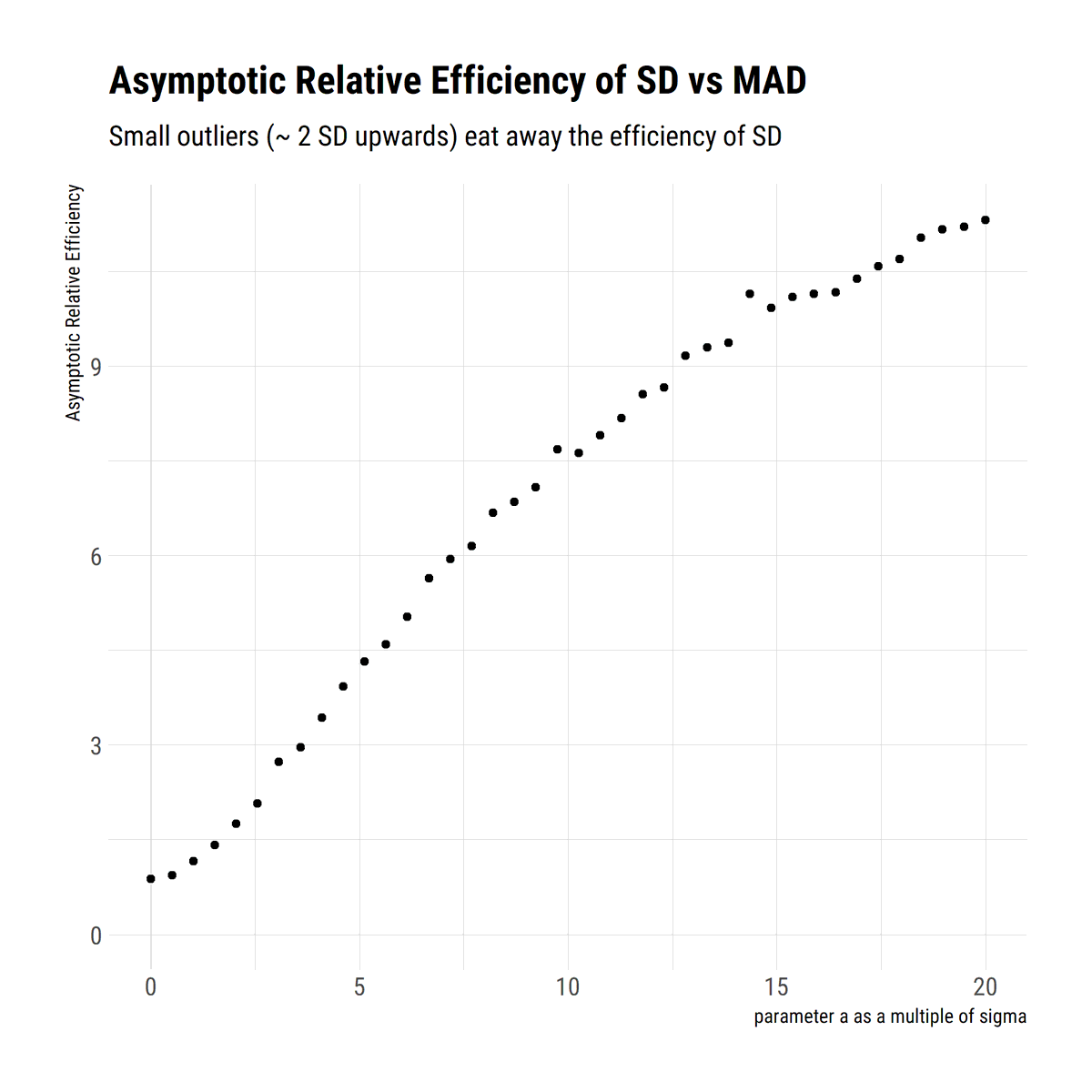
This highlights the problem with the tails. Tail probabilities are convex to errors in the scale. And for the scale itself we can easily produce bogus estimates. Thus, Black Swans can also acome from misinformation about what happens in the tail, even we are not in Extremistan.

Power Laws are ubiquitous. How can we intuitively understand the tail exponent? It is a measure of the rate of decay of the survival function. The lower alpha, the more slowly it decays, fatter the tail and the larger the influence of extreme events.

david-salazar.github.io/2020/05/19/und…

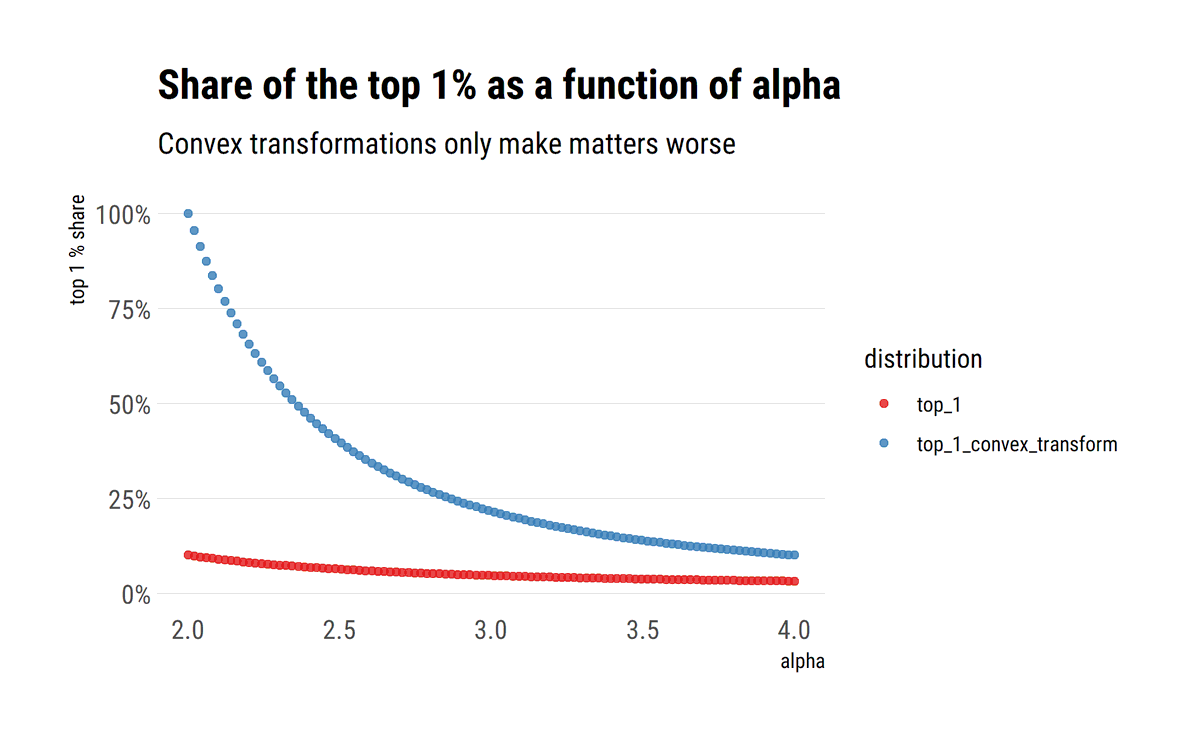
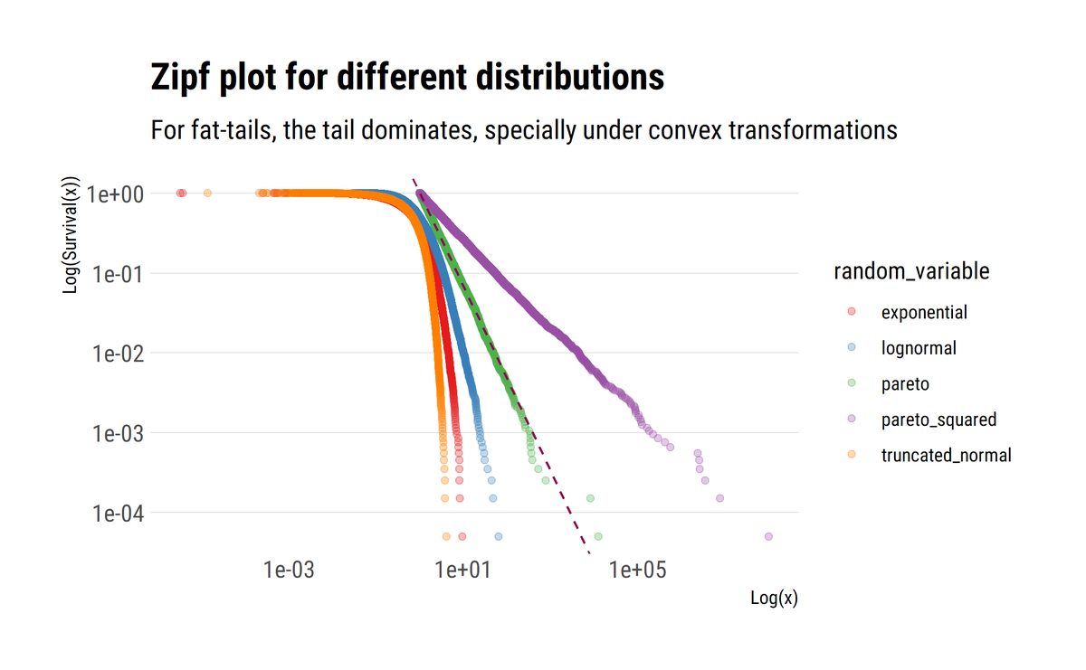
As @nntaleb shows, when the properties of the tail are scalable, the slope of the log of the surival function approaches $-\alpha$. Thus, mediocristan is where the decay of the tails approaches negative infinity. Also, convex transformations only worsen the decay of the tail.

For example, if wealth is Pareto distributed, the variance (sum of squares) of the wealth is going to be even more fat-tailed. This, again, comes from understanding how the tail exponent influences the tails.

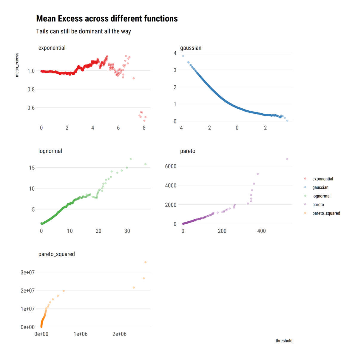
For comparison, @DrCirillo in his excellent YouTube lectures, studies the mean excess function E[X-v | X>v]. A weighted sum. In mediocristan, the weights decay quickly enough for the sum to decay with the threshold. In Extremistan, the sum is linearly increasing.

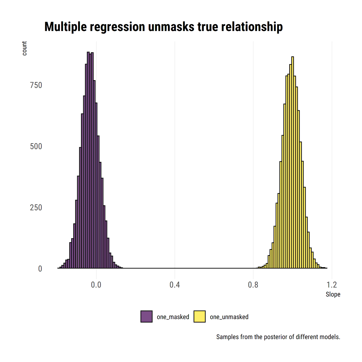
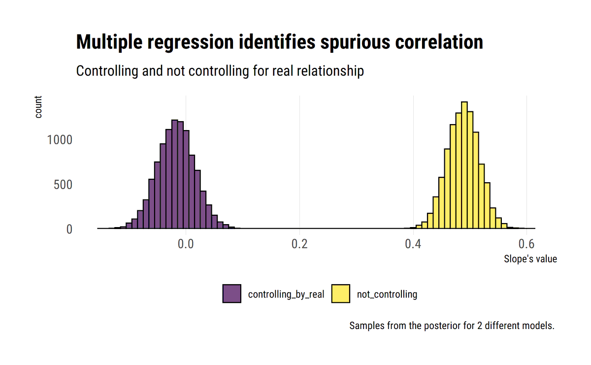
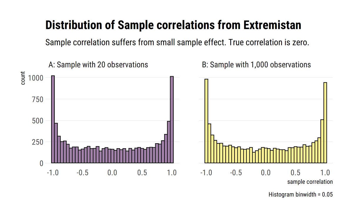
@nntaleb's take on correlation has a lot to unpack. Sample correlation is unreliable in Extremistan. However, even in Mediocristan, is routinley misunderstood and/or misued. Berkson's and Simpson's paradox, non-linearities, Mutual Information.

Blogpost: david-salazar.github.io/2020/05/22/cor…

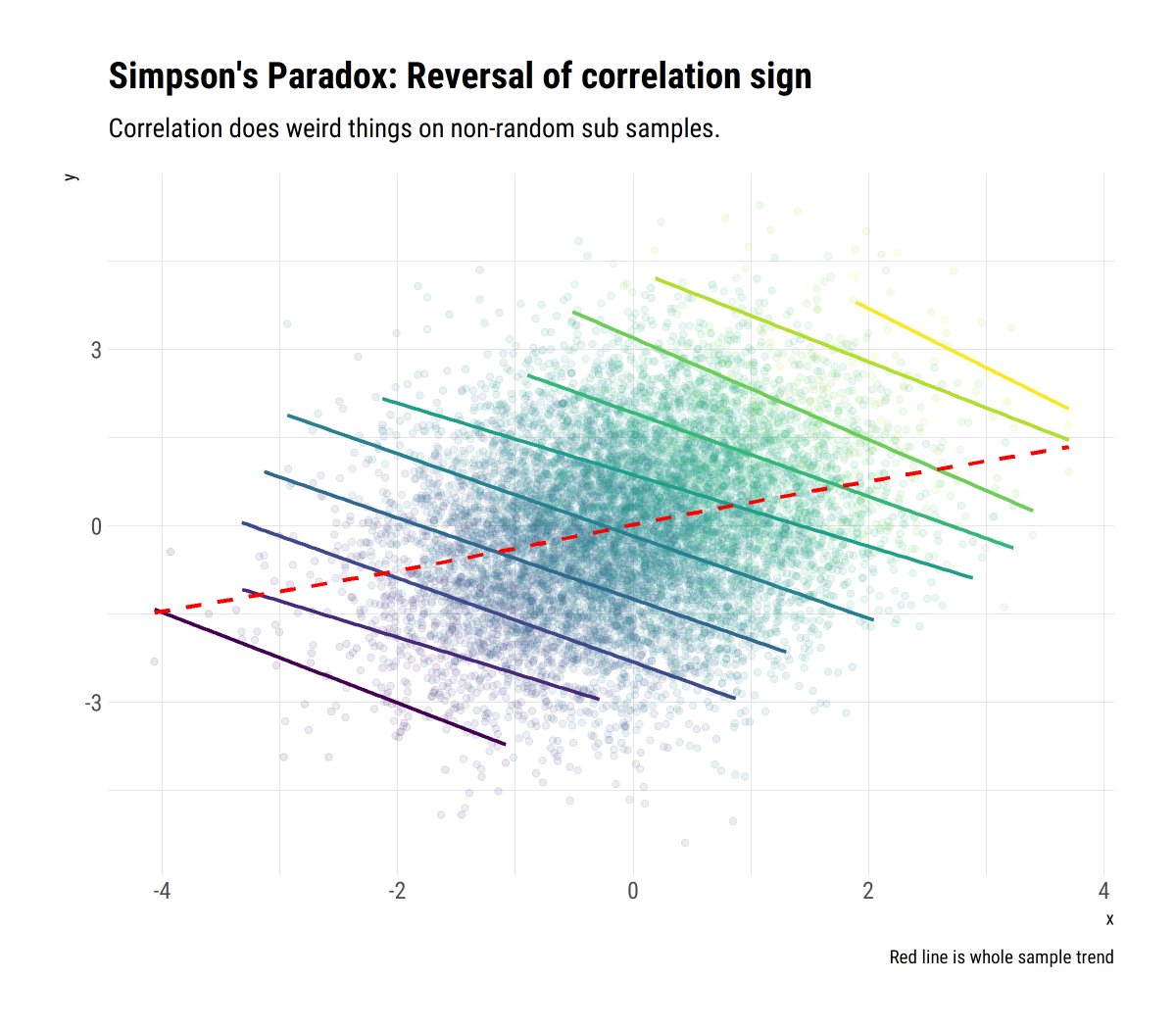
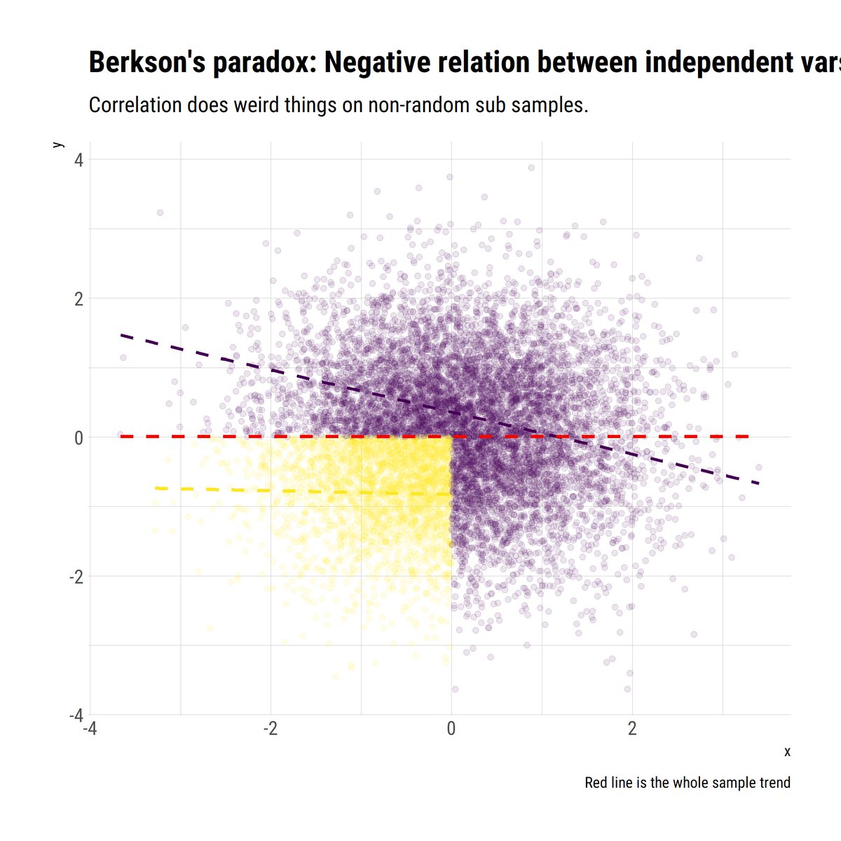
As Taleb says, a lot of paradoxes arise from a misunderstanding of correlation. For example, Simpson’s and Berkson’s paradoxes arise from mistakingly expecting the same correlation coefficient from the whole sample as in non-random subsamples from it.

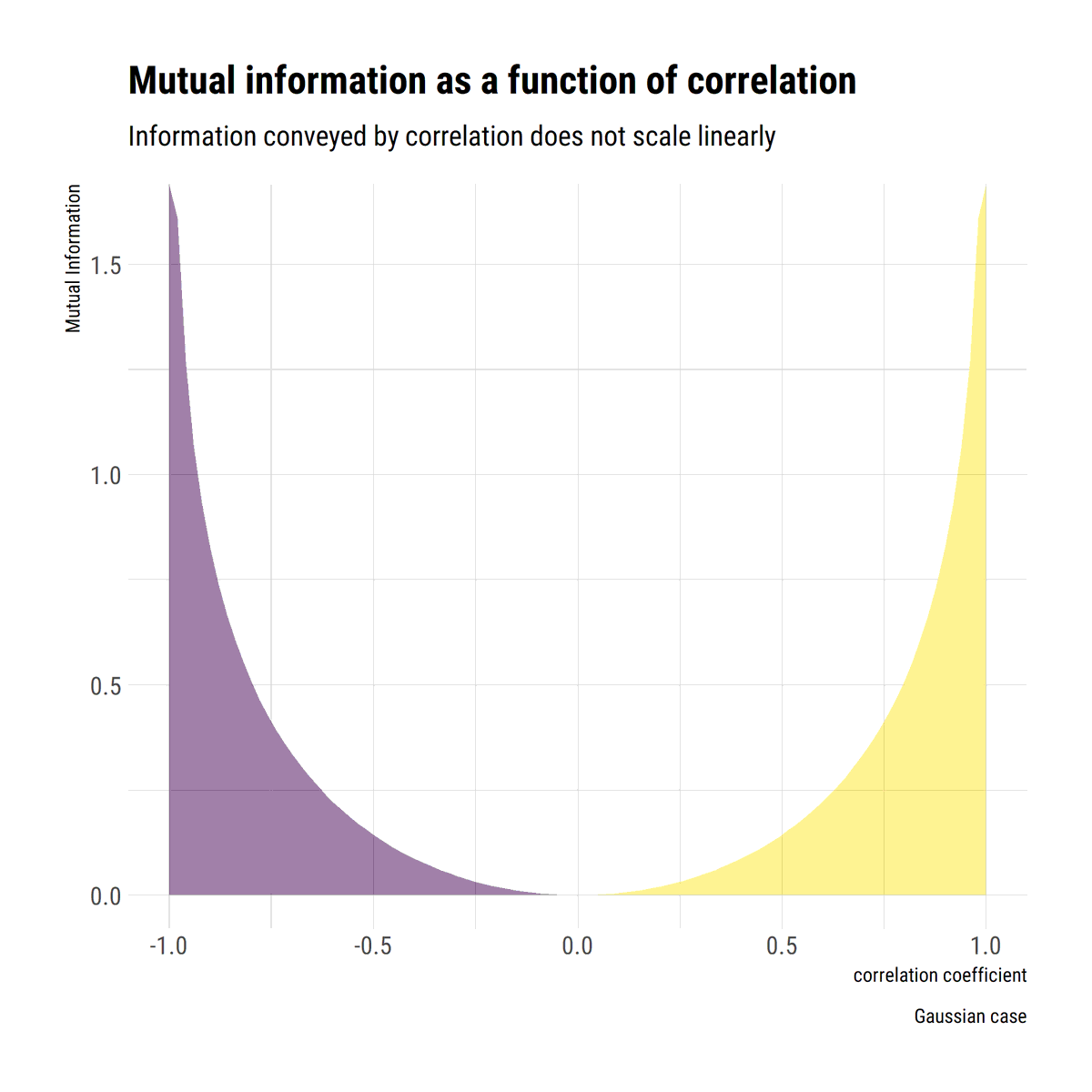
Perhaps more suprisingly, correlation should not be interpreted linearly. It picks up information about dependence; however, this signal does not scale linearly with the coefficient. A rho = 0.9 >>>> 0.7, whilst 0.5>0.3.

In Extremistan, even when the variance does not exist, the correlation coefficient can exist. However, the sample correlation is not useful for statistical purposes due to its slow convergence and large variance.

A thought experiment: You administer IQ tests to 10k people, then give them a “performance test” for anything, any task. 2000 of them are dead. Dead people score 0 on IQ and 0 on performance. The rest have the IQ uncorrelated to the performance What is the spurious correlation?

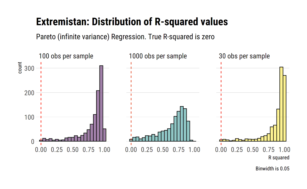
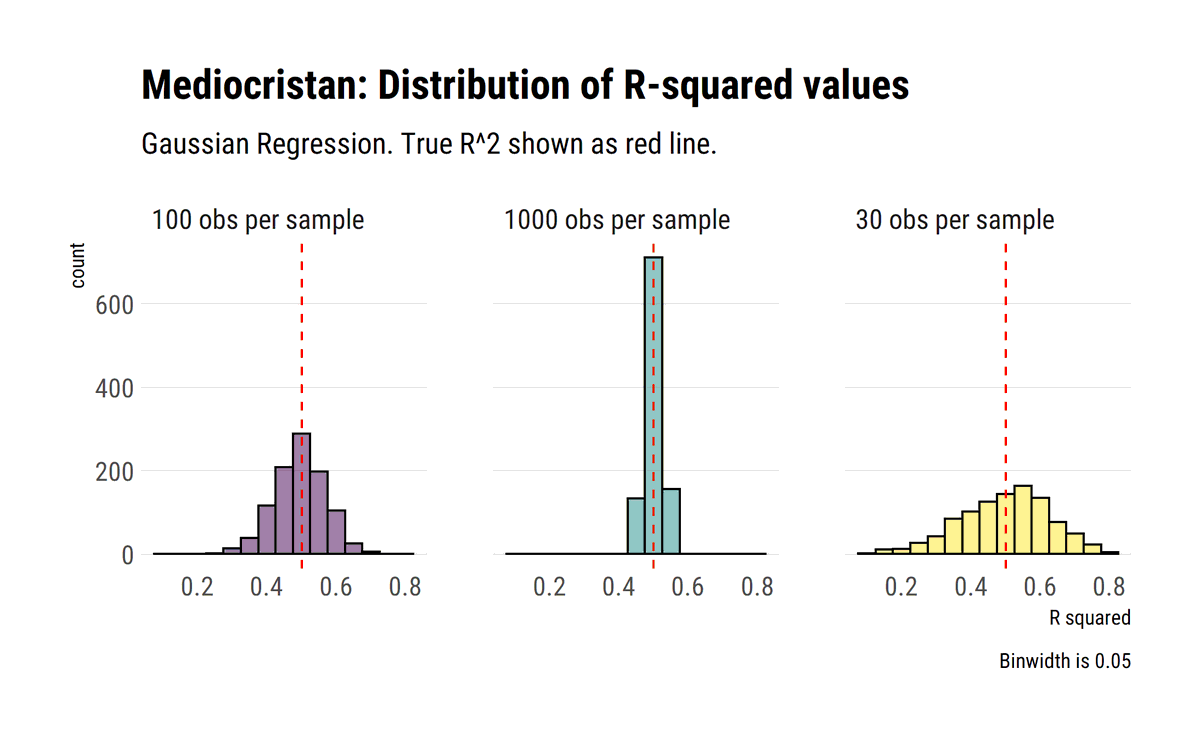
The turn of R^2 under fat tails. As @nntaleb says, when our outcome variable has infinite variance, our R^2 must be zero. Yet, almost always our data will say otherwise. R^2 becomes pure sample dependant noise #rstats

Monte-Carlo experiment:
david-salazar.github.io/2020/05/26/r-s…

The (slow) convergence of CLT. @nntaleb shows how the convergences varies preasymptotically across distributions. In Extremistan, the normal approximation is not warranted, even at very large samples sizes. #rstats

Blogpost with Monte-Carlo experiments:
david-salazar.github.io/2020/05/30/cen…

The LLN converges very slowly for fat-tailed variables. But it's even slower for its higher moments (see the max-to-sum gif). Beware "convergence": a single observation disproves it. Thus, @nntaleb is paranoid of invoking Mediocristan #rstats

Blogpost:
david-salazar.github.io/2020/06/02/lln…

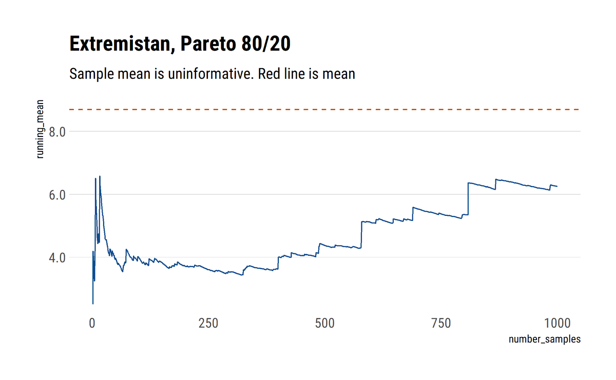
@nntaleb's kappa metric is a pre-asymptotic metric to answer the vital question in statistics: "how much data one needs to make meaningful statements about a given dataset?" It does this by measuring the rate of convergence of the scale of a partial sum as we add more summands

It's an operational metric that allows us to separate standard situations where both the LLN and the CLT work and the situation where they don't. Intuititvely, our sample mean will only stabilize when the partial sum is much larger than any possible instantiation of the r.v.

For mediocristan (think adding heights) this occurs pretty quickly. For extremsitan (think adding wealth) this takes an astronomically large n. For example, to get the same drop in variance as the Gaussian from n= 1 to n= 30, we need n > 10^9 for a Pareto 80/20!

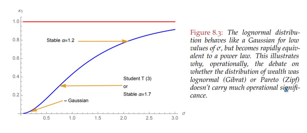
It also explains why the lognormal is neither thin-tailed nor fat-tailed. It's kappa metric depends entirely on the sd of the underlying normal. Do read chapter 8 of Statistical consequences of Fat Tails:
arxiv.org/ftp/arxiv/pape…

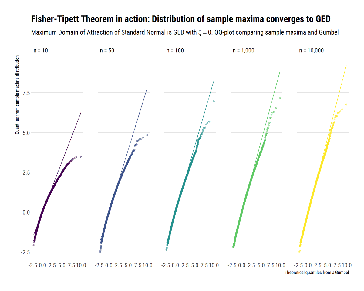
When the tail wags the dog, as @nntaleb says, one MUST think about the extremes. The Fisher-Tippet theorem is a type of CLT for (normalized) sample maxima. Here I try to use monte-carlo simulations to understand what this really means #rstats

Blogpost:
david-salazar.github.io/2020/06/10/fis…

Crucially, when the data is power law distributed, the sample maxima from this distribution will also be (asymptotically) power law distributed. That is, the maximum domain of attraction of a power law is always a Fréchet with the same tail index as the original power law:

Meanwhile, for distribution with exponential tails, for example the Gaussian, the Maximum Domain of Attraction is the Gumbel. However, the convergence is much slower. Thus, @nntaleb recommends using the exact distribution to work with the maxima of Gaussians.

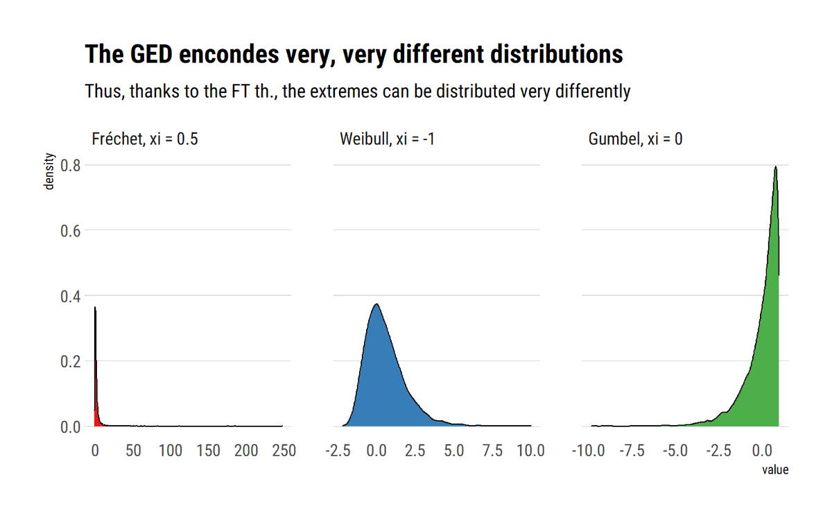
Finally, for light-tailed variables with an upper bound, the Maximum Domain of Attraction is the Weibull. For example, the standard uniform:

In a wonderful lecture, @DrCirillo shows how we can use the Pickands-Balkema-de Haan theorem to equivalently model the tails with the Generalized Pareto Distribution (ξ). Crucially, the GED and the GEP share the same ξ parameter.

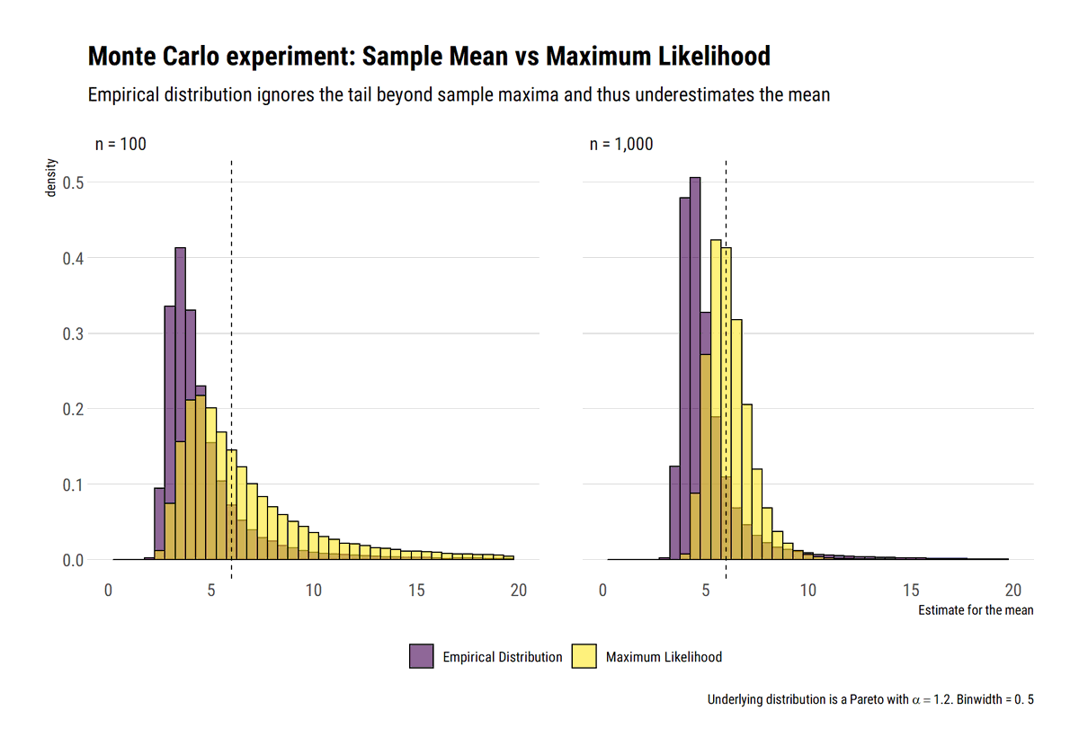
Under Extremistan, the "Empirical Distribution" fools us. Why? It cuts the tail at the sample maxima. Thus, a portion of the tail is hidden and ignored in our estimation. This hidden tail will bias all our estimates. The fatter the distribution, the most costly the mistake.

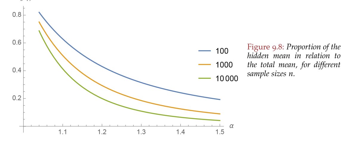
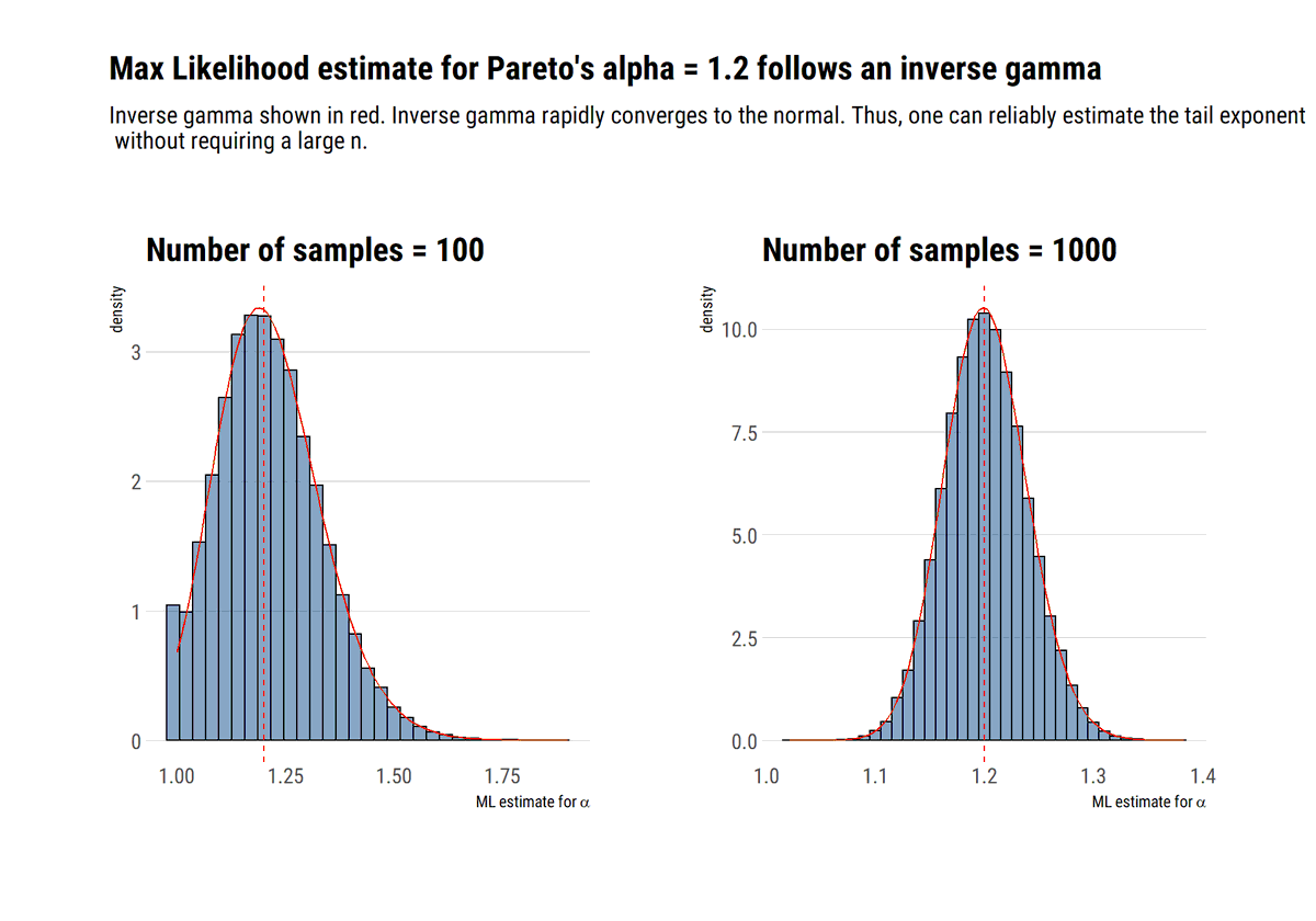
How to not get fooled by the empirical dist? Figure out the properties of the fat-tails and work with the distribution itself. Contrary to popular belief, one can figure out these properties with few data. For a pareto, max likelihood works very to estimate the tail exponent.

Why? @nntaleb shows that the ML estimator for alpha follows an inverse gamma which converges rapidly to a normal. Once we take into account the tail we plug in our alpha to for a less unreliable estimate of the mean #rstats

david-salazar.github.io/2020/06/11/how…

However, superiority over the “empirical distribution” is not that big of a compliment. No single point estimate can encompass the huge variation that fat-tails entail. The mean is hardly what matters.

A didactic example with real data to explore Extreme Value Theory? By an expert? @DrCirillo has you covered. Learn how to recognize fat-tails in real data and then model the extreme values #rstats

In financial time series there are volatility clusters. GARCHA models try to use this info by modeling the variance. Is this model, or any model that uses sample variance, warranted for the SP500? @nntaleb says no: its returns are too fat-tailed #rstats

david-salazar.github.io/2020/06/14/whe…

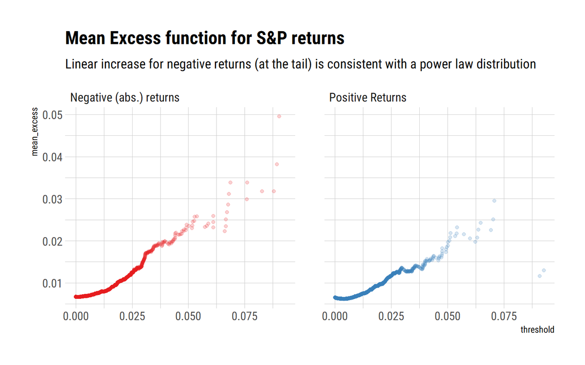
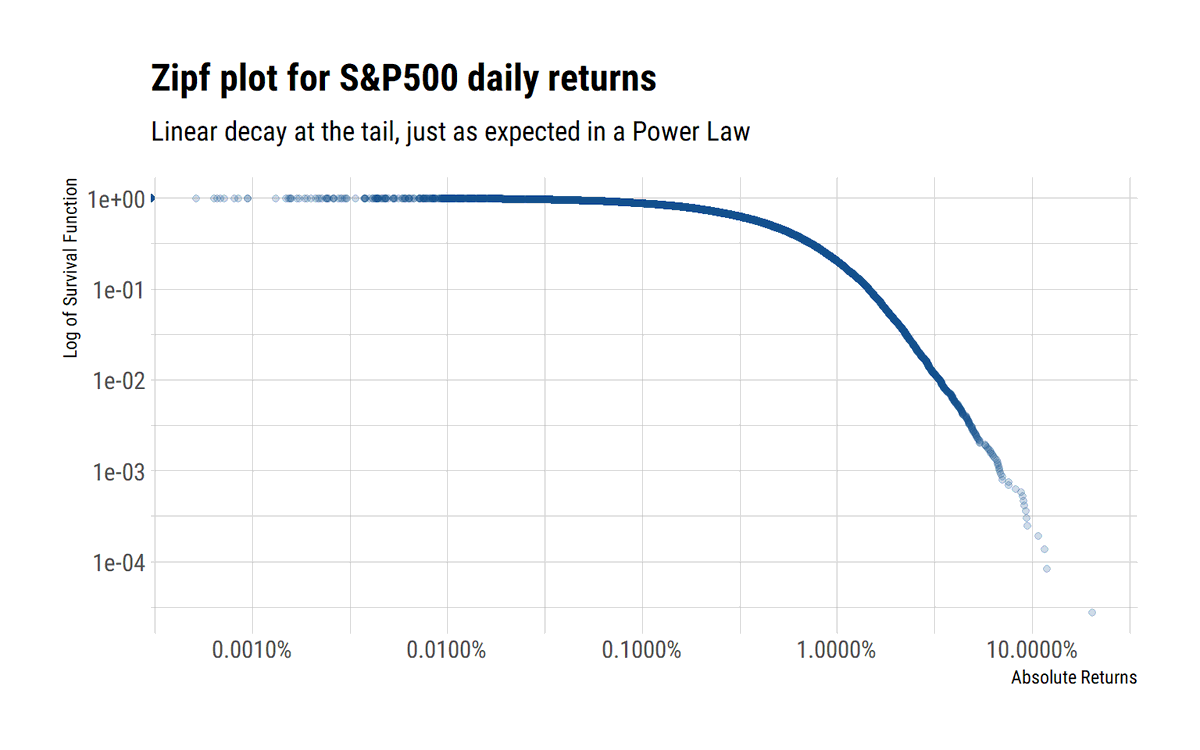
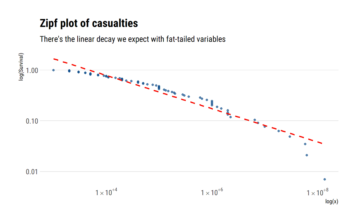
Above the Zipf plot and the mean excess plot show that the tail returns follow a Power-Law. We can reliably use the sample variance if and only if higher moments also exist. The max-to-sum ratio plot for the SP500 are telling enough:

A single point rejects this possibility.

In a great plot, Taleb shows the fundamental insight: SP500 is fat-tailed precisely due to the clustering of volatility. Kurtosis (in the long run, whatever that means) does not converge due to the serial dependence in the data. Thus, no Gaussian returns in the long run either.

The Fisher-Tippet theorem rests on the assumption of independence. However, the serial dependence in a time series renders this assumption untenable. Can we still use EVT to model the maxima of time series? The answer, it depends#rstats

david-salazar.github.io/2020/06/17/ext…

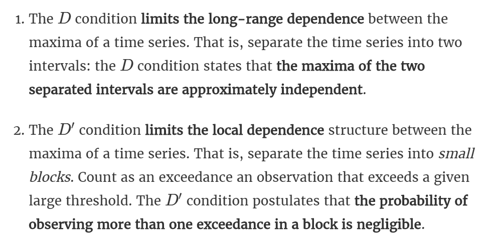
To model the maxima with EVT we must limit their dependence. Both the long-range dependence and the local dependence. These conditions are embedded in the so-called D conditions.

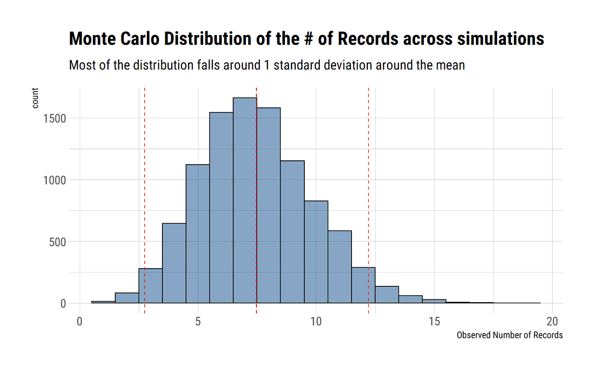
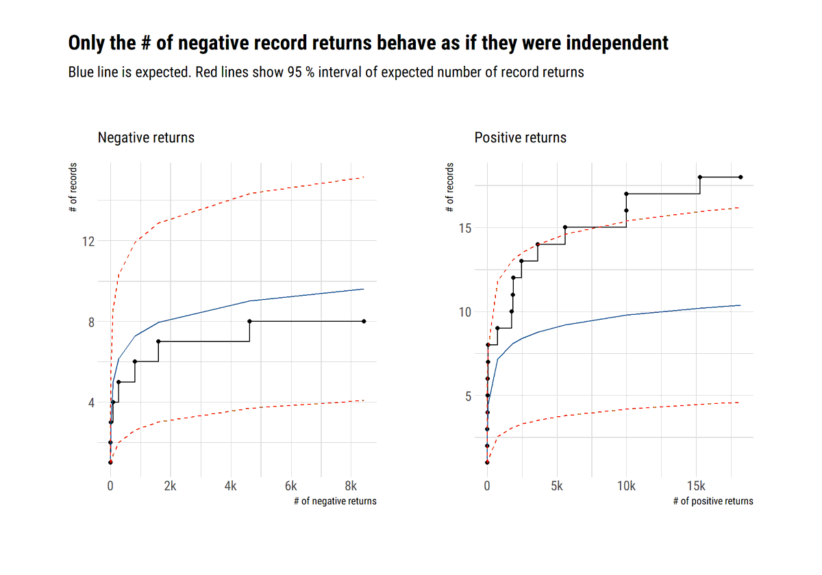
We can test for these conditions by comparing the number of record breaking observations in the data with the expected number of record breaking observations if the observations were independent.
@nntaleb shows that SP500 negative returns can be considered independent

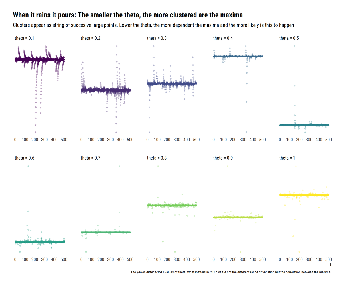
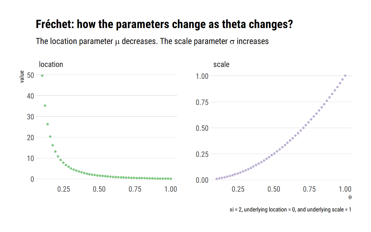
Once we've tested for these conditions, we can generaliza the Fisher Tippet Theorem: the maxima of a time series has the same Maximum Domain of Attraction as independent observations with the same marginal. However, the distribution is raised to a power: the extremal index

The extremal index (θ) is a measure of the clustering of the maxima. The lower the theta, the more clustered are the maxima. What does this mean? When it rains, it pours. The tail events all come together for dependent time series. Here a Cauchy AR(1): a string of high obs.

Finally, ignoring these clustering leads to underestimating the quantiles of the distribution. The VaR for a given confidence level for independence observations is higher than for dependent observations. Nevertheless, when the tail event happens, lots of others accompany it.

Probability calibration is a way evaluating forecasts. Is this truly the mark of a good analysis? Under fat-tails, @nntaleb says NO! Calibration amounts to binary payoff that cannot possibly track the variability of fat-tailed variables #rstats

david-salazar.github.io/2020/06/24/pro…

binary payoff: a fixed sum is paid off if the event happens. Hedge the risk of a fat-tailed variable? which lump sum? there is no possible lump sum that can hedge the exposure to a fat-tailed variable.

Why? The reason is the same as to why single-point forecasts are useless: There is no typical collapse or disaster, owing to the absence of characteristic scale. Conditional on a large loss, an even larger loss is always possible #rstats

Therefore, one cannot know in advance the size of the collapse nor how much the lump sum should be. That is, reducing the variability of a fat-tailed random variable to a binary payoff makes no sense. Therefore, probability calibration with fat-tailed variables makes no sense.

Now it's the turn of the Gini Index under fat-tails: intuitively, the empirical distribution underestimates the tail and thus the non-parametric version of the estimator underestimates it. What to do? #rstats

david-salazar.github.io/2020/06/26/gin…

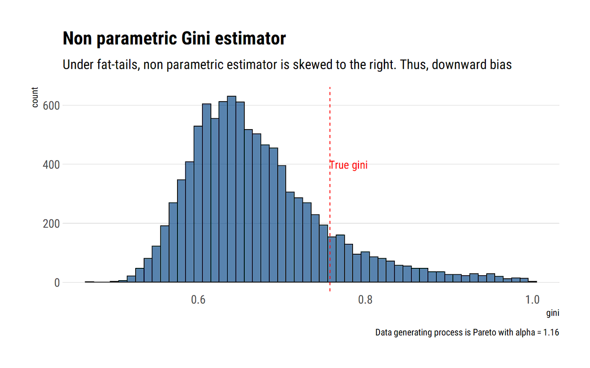
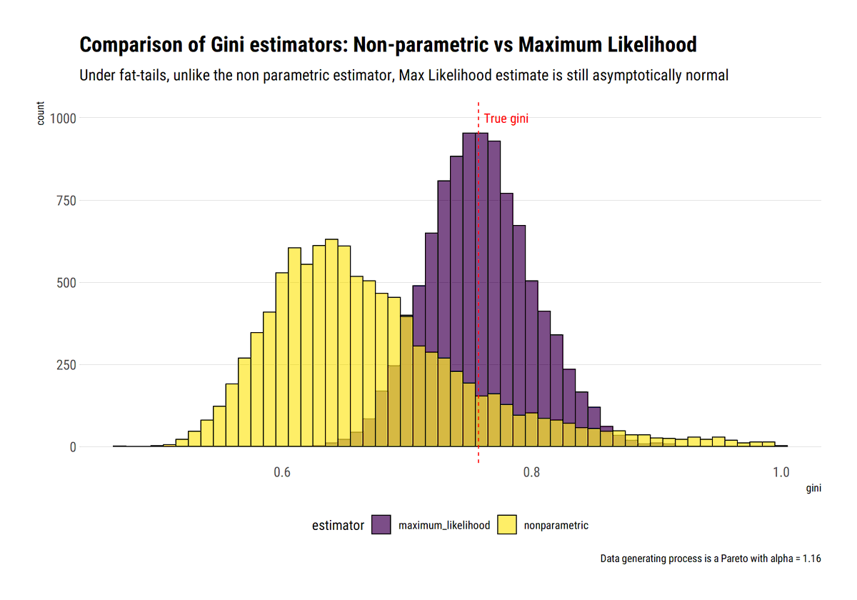
As @nntaleb says, account for the tail properties first, which as we've seen can be done with few data and Maximum Likelihood (ML). Then, estimate Gini with plug-in estimator. This ML estimator is asymptotically normal and efficient.

Re-implementing @nntaleb and @DrCirillo's paper in #rstats and using @mcmc_stan . Casualties from pandemics are patently fat-tailed. How do they prove it? Graphical analysis and Extreme Value Theory supply the distributional evidence

david-salazar.github.io/2020/07/05/tai…

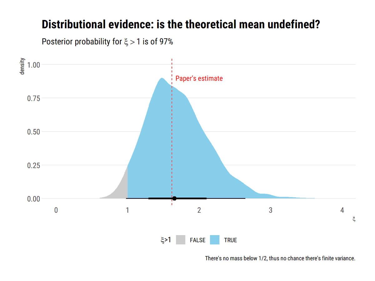
The graphical analysis show that there's a huuuge array of variation (histogram below) and the tail decays very slowly (zipf plot and mean excess). The end result: the theoretical moments are likely undefined: in the max-to-sum ratio plot, none of the moments converges

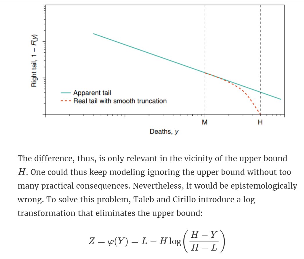
Wait a moment? Infinite casualties. There's an upper bound (total population) that conflicts with these infinite moments @nntaleb and @DrCirillo introduce a log transformation that eliminates the upper bound by introducing dual observations.

EVT gives us the tool to know how fat are the tails: we approximate the deep tail with a Generalized Pareto Distribution. The larger \xi, the fatter the distribution. The posterior distribution for \xi is overwhelming:

What does this mean? Given the fat-tailedness of the data and the resulting lack of characteristic scale from the huge array of variability that it’s relevant, there’s no possibility of forecasting what we may face with either a pointwise prediction or a distributional forecast.

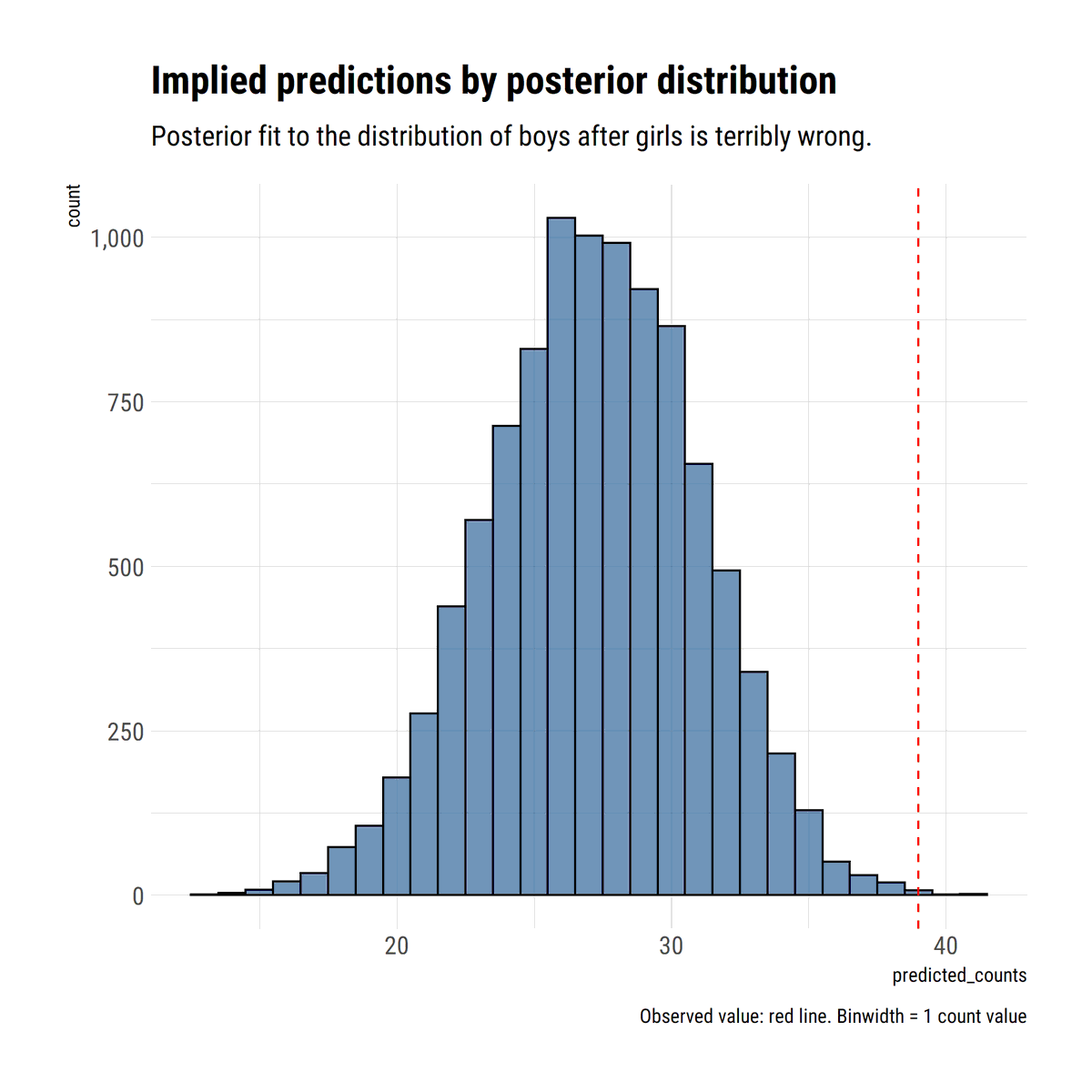
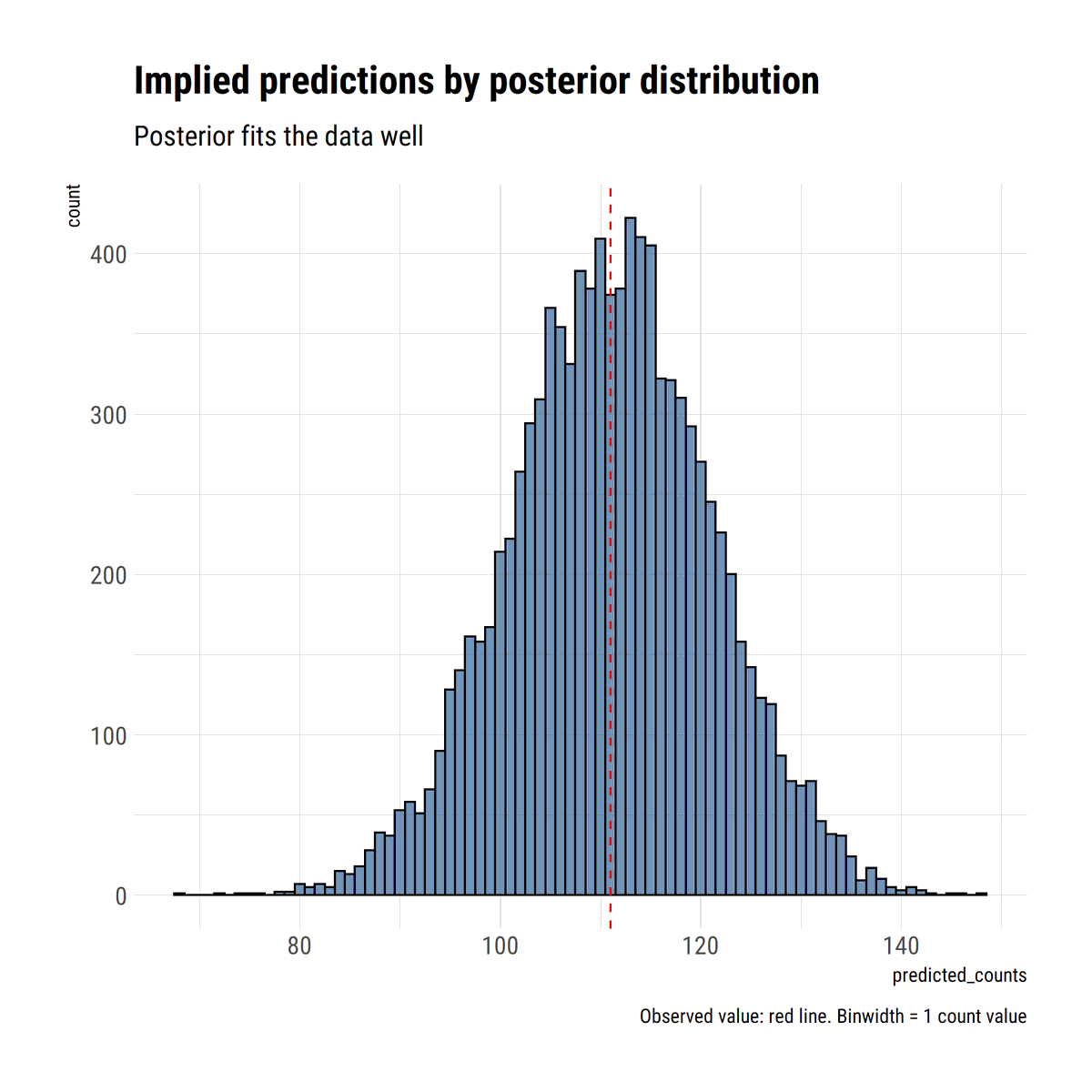
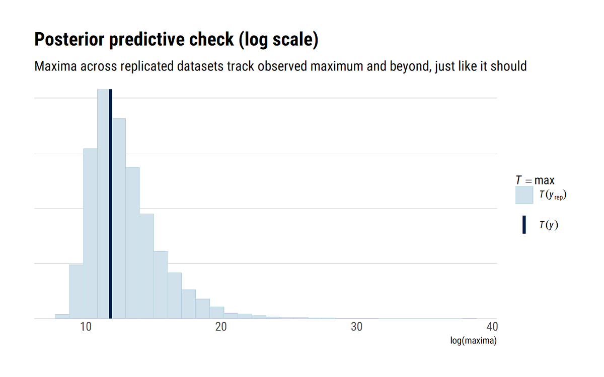
This is evident with a posterior predictive check: we replicate the data according to our model. what about the replicated maxima? These definitely should include the observed maxima: but also much larger values. That is the whole point of being in the MDA of a Fréchet (xi>0)

That is, the distributional evidence is there! At any point in the pandemic, all we can say is that it can get much worse. Given the asymmetric risks that we face, Taleb's incerto is very clear: eliminate our exposure as swifltly as we can. Or @yaneerbaryam's way: get to 0 now!

They also stress their data quite heavily: both with measurement error and altogether removal of observations with resampled versions of their data, I incorporate measurement error in a bayesian way and find the same: the results still hold.

It's a short, fun and important paper. Read it!

nature.com/articles/s4156…

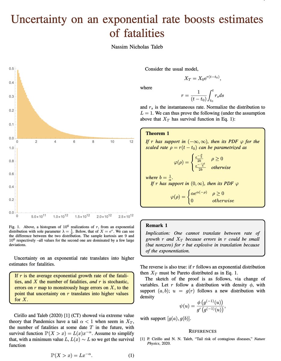
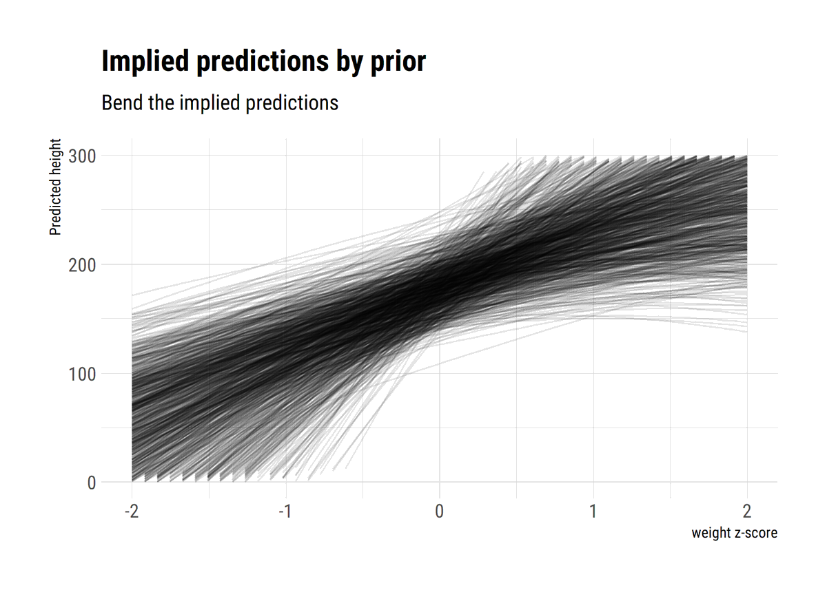
We can also arrive at maximal uncertainty with an a priori argument @nntaleb shows that given exponential growth, uncertainty in the rate of growth translates into maximal uncertainty around the number of casualties. Remember, uncertainty loves convexity.