What do polar coordinates, polar matrix factorization, & Helmholz decomposition of a vector field have in common?
They’re all implied by Brenier’s Theorem: a cornerstone of Optimal Transport theory. It’s a fundamental decomposition result & rly deserves to be better known.
1/7
They’re all implied by Brenier’s Theorem: a cornerstone of Optimal Transport theory. It’s a fundamental decomposition result & rly deserves to be better known.
1/7

Brenier's Thm ('91): A non-degenerate vector field
u: Ω ∈ ℝⁿ → ℝⁿ has a unique decomposition
u = ∇ϕ∘s
where ϕ is a convex potential on Ω, and s is measure-preserving (think density → density).
Here s is a multi-dimensional “rearrangement” (a sort in 1D)
2/7
u: Ω ∈ ℝⁿ → ℝⁿ has a unique decomposition
u = ∇ϕ∘s
where ϕ is a convex potential on Ω, and s is measure-preserving (think density → density).
Here s is a multi-dimensional “rearrangement” (a sort in 1D)
2/7
In optimal transport, Brenier's thm implies existence, uniqueness & monotonicity of an OT map w.r.t L₂ cost, between two given densities p(x) & q(y). Let
u: ℝⁿ → ℝⁿ & c(x,y) = ‖x − y‖²,
Optimal map u = ∇ϕ taking p to q where ϕ is convex.
3/7
u: ℝⁿ → ℝⁿ & c(x,y) = ‖x − y‖²,
Optimal map u = ∇ϕ taking p to q where ϕ is convex.
3/7
https://twitter.com/gabrielpeyre/status/1147732031566155776?s=20
Brenier proved a weaker result in '87 in a manuscript in French, but later in '91 published the definitive version in Comms. on Pure and Applied Maths.
* It's a wonderful paper and well-worth reading on its own merit & to learn the special cases *
citeseerx.ist.psu.edu/viewdoc/downlo…
4/7
* It's a wonderful paper and well-worth reading on its own merit & to learn the special cases *
citeseerx.ist.psu.edu/viewdoc/downlo…
4/7

Like any great idea, it was (sort of) scooped. But luckily others were in faraway fields & less general
One was in weather forecasting, other in statistics:
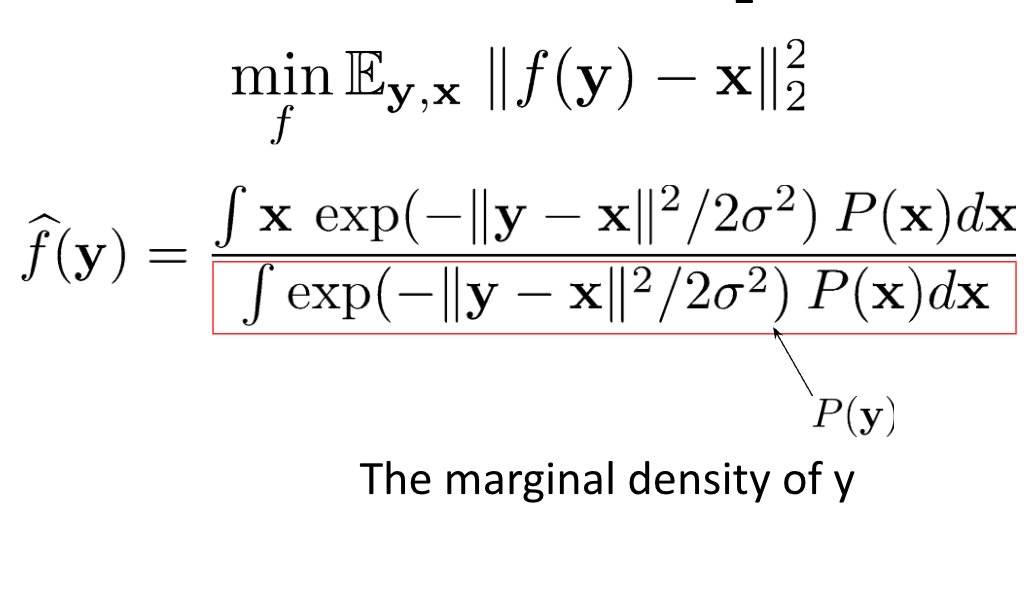
Given x and y w/ densities p(x), q(y) find a function
y = f(x) that maximizes 𝔼(xy)
Soln: f =∇ϕ for some convex ϕ
5/7
One was in weather forecasting, other in statistics:
Given x and y w/ densities p(x), q(y) find a function
y = f(x) that maximizes 𝔼(xy)
Soln: f =∇ϕ for some convex ϕ
5/7

What if the data live on a manifold?
Well, for this case there's a very cool generalization of Brenier's result by McCann, where the magical exponential maps makes an appearance.
(Amazing that this paper is still just a preprint 20 yrs on!)
mis.mpg.de/preprints/1999…
6/7
Well, for this case there's a very cool generalization of Brenier's result by McCann, where the magical exponential maps makes an appearance.
(Amazing that this paper is still just a preprint 20 yrs on!)
mis.mpg.de/preprints/1999…
6/7

The importance of Brenier's Thm has only grown recently in Machine Learning and Statistics.
Not only is it a cornerstone of optimal transport generally, but it is also being deployed in recent works addressing "potential flows."
7/7 Fin
Not only is it a cornerstone of optimal transport generally, but it is also being deployed in recent works addressing "potential flows."
7/7 Fin

• • •
Missing some Tweet in this thread? You can try to
force a refresh