Data similarity has such a simple visual interpretation that it will light all the bulbs in your head.
The mathematical magic tells you that similarity is given by the inner product. Have you thought about why?
This is how elementary geometry explains it all.
↓ A thread. ↓
The mathematical magic tells you that similarity is given by the inner product. Have you thought about why?
This is how elementary geometry explains it all.
↓ A thread. ↓

Let's start in the beginning!
In machine learning, data is represented by vectors. So, instead of observations and features, we talk about tuples of (real) numbers.
In machine learning, data is represented by vectors. So, instead of observations and features, we talk about tuples of (real) numbers.

Vectors have two special functions defined on them: their norms and inner products. Norms simply describe their magnitude, while inner products describe
.
.
.
well, a 𝐥𝐨𝐭 of things.
Let's start with the fundamentals!
.
.
.
well, a 𝐥𝐨𝐭 of things.
Let's start with the fundamentals!
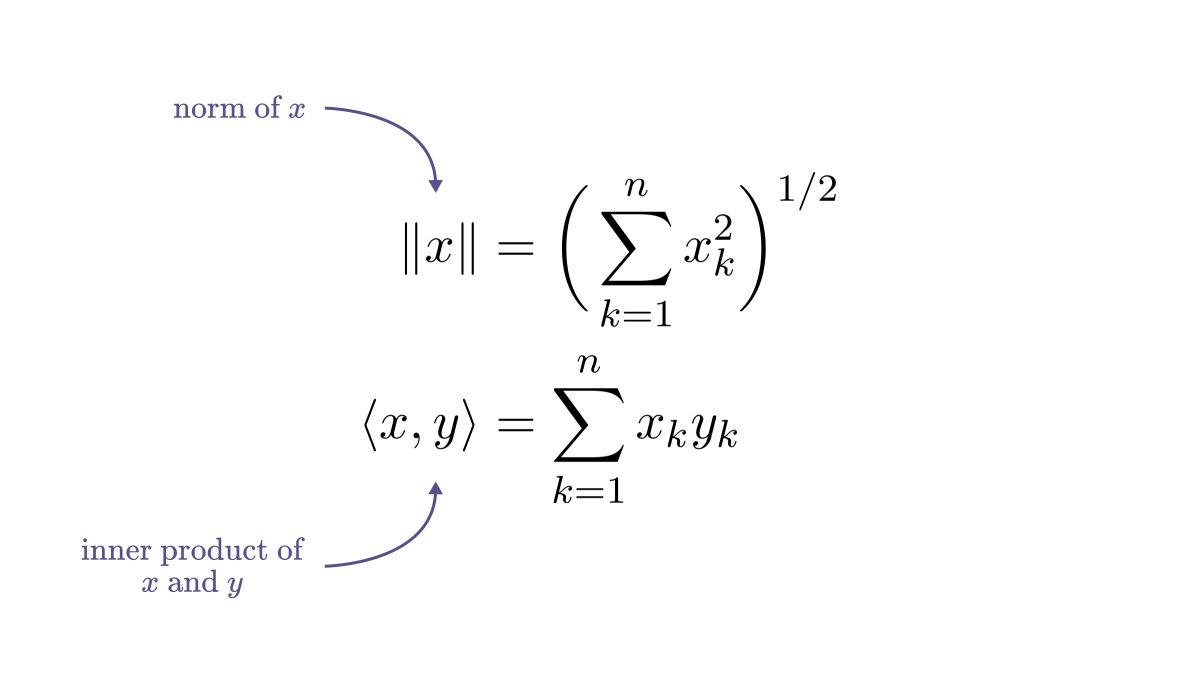
First of all, the norm can be expressed in terms of the inner product.
Moreover, the inner product is linear in both variables. (Check these by hand if you don't believe me.)
Bilinearity gives rise to a geometric interpretation of the inner product.
Moreover, the inner product is linear in both variables. (Check these by hand if you don't believe me.)
Bilinearity gives rise to a geometric interpretation of the inner product.

If we form an imaginary triangle from 𝑥, 𝑦, and 𝑥+𝑦, we can express the inner product in terms of the sides' length.
(Even in higher dimensions, we can form this triangle. It'll be just on a two-dimensional subspace.)
(Even in higher dimensions, we can form this triangle. It'll be just on a two-dimensional subspace.)

However, applying the law of cosines, we obtain yet another way of expressing the length of 𝑥+𝑦, this time in terms of the other sides and the angle enclosed by them.

(If you need to catch up on the law of cosines, check out the Wikipedia page here: en.wikipedia.org/wiki/Law_of_co…)
Putting these together, we see that the inner product of 𝑥 and 𝑦 is the product of
• the norm of 𝑥,
• the norm of 𝑦,
• and the cosine of their enclosed angle!
• the norm of 𝑥,
• the norm of 𝑦,
• and the cosine of their enclosed angle!

If we scale down 𝑥 and 𝑦 to unit lengths, their inner product simply gives the cosine of the angle.
You might know this as cosine similarity.
For data points, the closer it is to 1, the more the features move together.
You might know this as cosine similarity.
For data points, the closer it is to 1, the more the features move together.

Inner products play an essential part in data science and machine learning.
Because of this, they are the main topic of the newest chapter of my book, The Mathematics of Machine Learning. Each week, I release a new chapter, just as I write them.
tivadar.gumroad.com/l/mathematics-…
Because of this, they are the main topic of the newest chapter of my book, The Mathematics of Machine Learning. Each week, I release a new chapter, just as I write them.
tivadar.gumroad.com/l/mathematics-…
I post several threads like this every week, diving deep into concepts in machine learning and mathematics.
If you have enjoyed this, make sure to follow me and stay tuned for more!
The theory behind machine learning is beautiful, and I want to show this to you.
If you have enjoyed this, make sure to follow me and stay tuned for more!
The theory behind machine learning is beautiful, and I want to show this to you.
• • •
Missing some Tweet in this thread? You can try to
force a refresh