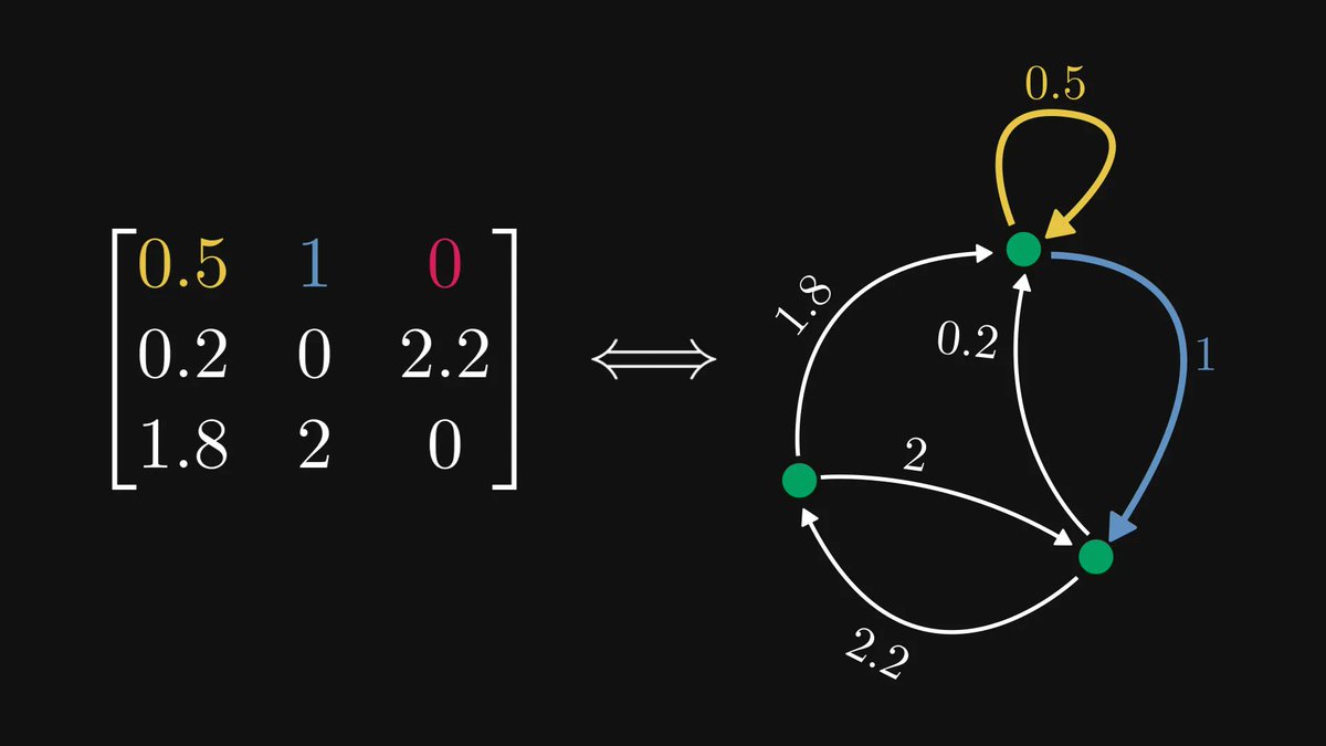
There is more than one way to think about matrix multiplication.
By definition, it is not easy to understand. However, there are multiple ways of looking at it, each one revealing invaluable insights.
Let's take a look at them!
↓ A thread. ↓
By definition, it is not easy to understand. However, there are multiple ways of looking at it, each one revealing invaluable insights.
Let's take a look at them!
↓ A thread. ↓

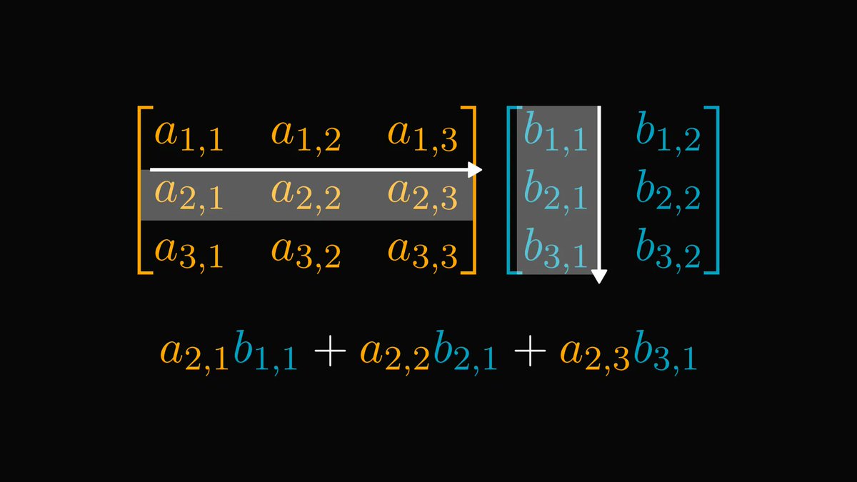
First, let's unravel the definition and visualize what happens.
For instance, the element in the 2nd row and 1st column of the product matrix is created from the 2nd row of the left and 1st column of the right matrices by summing their elementwise product.
For instance, the element in the 2nd row and 1st column of the product matrix is created from the 2nd row of the left and 1st column of the right matrices by summing their elementwise product.

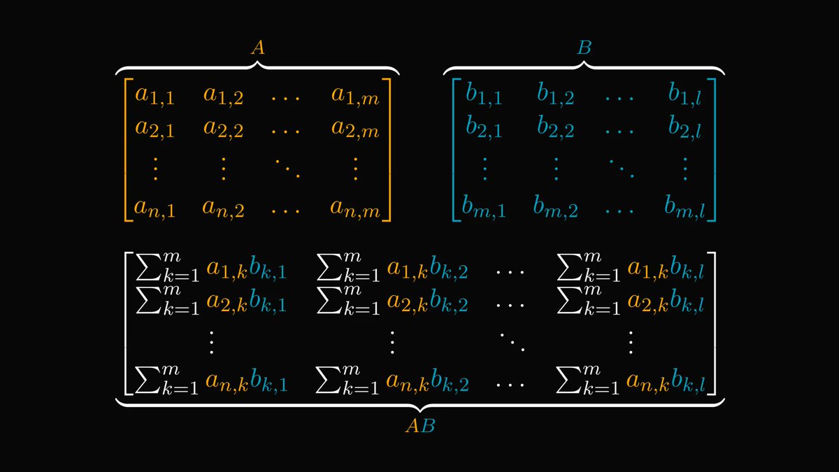
To move beyond the definition, let's introduce some notations.
A matrix is built from rows and vectors. These can be viewed as individual vectors.
You can think of them as a horizontal stack of column vectors or a vertical stack of row vectors.
A matrix is built from rows and vectors. These can be viewed as individual vectors.
You can think of them as a horizontal stack of column vectors or a vertical stack of row vectors.

Let's start by multiplying a matrix and a row vector.
By writing out the definition, it turns out that the product is just a linear combination of the columns, where the coefficients are determined by the vector we are multiplying with!
By writing out the definition, it turns out that the product is just a linear combination of the columns, where the coefficients are determined by the vector we are multiplying with!

Taking this one step further, we can stack another vector.
This way, we can see that the product of an (n x n) and an (n x 2) matrix equals the product of the left matrix and the columns of the right matrix, horizontally stacked.
This way, we can see that the product of an (n x n) and an (n x 2) matrix equals the product of the left matrix and the columns of the right matrix, horizontally stacked.

Applying the same logic, we can finally see that the product matrix is nothing else than the left matrix times the columns of the right matrix, horizontally stacked.
This is an extremely powerful way of thinking about matrix multiplication.
This is an extremely powerful way of thinking about matrix multiplication.

We can also get the product as vertically stacked row vectors by switching our viewpoint a bit.

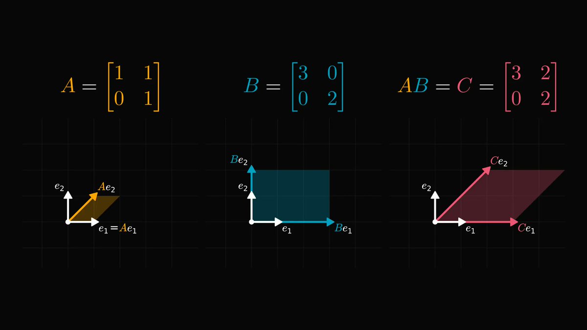
There is another interpretation of matrix multiplication.
Let's rewind and go back to the beginning, studying the product of a matrix 𝐴 and a column vector 𝑥.
Do the sums in the result look familiar?
Let's rewind and go back to the beginning, studying the product of a matrix 𝐴 and a column vector 𝑥.
Do the sums in the result look familiar?

These sums are just the dot product of the row vectors of 𝐴, taken with the column vector 𝑥!

In general, the product of 𝐴 and 𝐵 is simply the dot products of row vectors from 𝐴 and column vectors from 𝐵!

To sum up, we have three interpretations: matrix multiplication as
1. vertically stacking row vectors,
2. horizontally stacking column vectors,
3. and as dot products of row vectors with column vectors.
When studying matrices, each of them is immensely useful.
1. vertically stacking row vectors,
2. horizontally stacking column vectors,
3. and as dot products of row vectors with column vectors.
When studying matrices, each of them is immensely useful.

Having a deep understanding of math will make you a better engineer. I want to help you with this, so I am writing a comprehensive book about the subject.
If you are interested in the details and beauties of mathematics, check out the early access!
tivadardanka.com/book
If you are interested in the details and beauties of mathematics, check out the early access!
tivadardanka.com/book
If you have enjoyed this thread, consider giving it a retweet and following me!
I regularly post deep-dive explanations about seemingly complex concepts from mathematics and machine learning.
Mathematics is beautiful, and I want to show this to you.
I regularly post deep-dive explanations about seemingly complex concepts from mathematics and machine learning.
Mathematics is beautiful, and I want to show this to you.
• • •
Missing some Tweet in this thread? You can try to
force a refresh