Thread by @keenanisalive

Models in engineering & science have *way* more complexity in geometry/materials than what conventional solvers can handle.

But imagine if simulation was like Monte Carlo rendering: just load up a complex model and hit "go"; don't worry about meshing, basis functions, etc. [1/n]

Our #SIGGRAPH2022 paper takes a major step toward this vision by building a bridge between PDEs & volume rendering: cs.dartmouth.edu/wjarosz/public…

Joint work with
@daseyb — darioseyb.com
@rohansawhney1 — rohansawhney.io
@wkjarosz — cs.dartmouth.edu/wjarosz/

[2/n]

Here's one fun example: heat radiating off of infinitely many aperiodically-arranged black body emitters, each with super-detailed geometry, and super-detailed material coefficients.

From this view alone, the *boundary* meshes have ~600M vertices. Try doing that with FEM! [3/n]

To get the same level of detail with FEM—even for a tiny piece of the scene—we need about 8.5 million tets & 2.5 hours of meshing time.

With Monte Carlo we get rapid feedback, even if geometry or materials change (above it's even implemented in a GLSL fragment shader!)

[4/n]

At this moment the experts in the crowd will ask, "what about boundary element methods?" and "have you heard of meshless FEM?"

The short story is: these methods must still do (very!) tough, expensive, & error-prone node placement, global solves, etc. (See paper for more.) [5/n]

Our journey with Monte Carlo began a few years ago, when we realized that rendering techniques from computer graphics could be used to turbo charge Muller's little known "walk on spheres" algorithm for solving PDEs. You can read all about it here:

https://twitter.com/keenanisalive/status/1258152669727899650

[6/n]

Our latest paper makes the connection between rendering & simulation even stronger, by linking tools from volume rendering to ideas in stochastic calculus.

We can hence apply techniques for heterogeneous media (clouds, smoke, …) to PDEs with spatially-varying coefficients [7/n]

Spatially-varying coefficients are essential for capturing the rich material properties of real-world phenomena.

Want to understand the thermal or acoustic performance of a building? Even a basic wall isn't a homogenous slab—it has many layers of different density, etc. [8/n]

And that's just the tip of the iceberg—PDEs with spatially-varying coefficients are everywhere in science & engineering! From antenna design, to biomolecular simulation, to understanding groundwater pollution to… you name it

How can we simulate systems of this complexity? [9/n]

A major challenge in any PDE solver is "spatial discretization": whether you use finite differences or FEM or BEM or… whatever, you have to break up space into little pieces in order to simulate it. This process is expensive & error prone—especially for complex systems! [10/n]

Apart from just the massive cost of discretization/meshing, it causes two major headaches for solving PDEs:

1. important geometric features get destroyed, and
2. you get aliasing in the functions describing your problem (boundary conditions, PDE coefficients, etc.).

[11/n]

Because spatial discretization is such a pain in the @#$%, folks in photorealistic rendering moved away from meshing many years ago—and toward Monte Carlo methods which only need pointwise access to geometry (via ray-scene intersection queries).

So, what about PDEs? [12/n]

Here there's a little-known algorithm called "walk on spheres (WoS)," which avoids the problem of spatial discretization altogether.

Much like rendering, all it needs to know is the closest boundary point x' for any given point x. Details here:

https://twitter.com/keenanisalive/status/1258152687130083333

[13/n]

Now, to be candid: WoS is *way* behind mature technology like finite element methods (FEM) in terms of the kinds of problems it can handle (…so far!)

Especially in graphics we've seen amaaaaazing PDE solvers that handle wild, complex, multi-physics scenarios—like pizza! [14/n]

But the WoS idea—and its promise to free us from the bonds of spatial discretization—is so alluring that we have taken up the mission of expanding WoS to broader & broader classes of PDEs.

So, let's talk about how we can extend WoS to variable-coefficient PDEs. [15/n]

This story is really a tale of three kinds of equations:

* partial differential equations (PDE)
* integral equations (IE)
* stochastic differential equations (SDE)

Our paper (Sections 2 & 4) provides a sort of "playbook" of how to convert between these different forms.

[16/n]

In precise terms, our goal is to develop a WoS method that solves 2nd order linear elliptic equations with spatially-varying diffusion, drift, and absorption coefficients.

Let's unpack this jargon term by term. [17/n]

First: PDEs describe phenomena by relating rates of change. E.g., the 1D heat equation says the change in temperature over time is proportional to its 2nd derivative in space: ∂u/∂t = ∂² u/∂x².

To get the temperature itself, we have to solve for u—usually numerically! [18/n]

"2nd order" means there are at most two derivatives in space; "linear" means derivatives are combined in a linear way (e.g., not squared or multiplied together). "Elliptic" roughly means the solution at each point sort of looks like a (weighted) average of nearby values [19/n].

Seeing some examples is helpful.

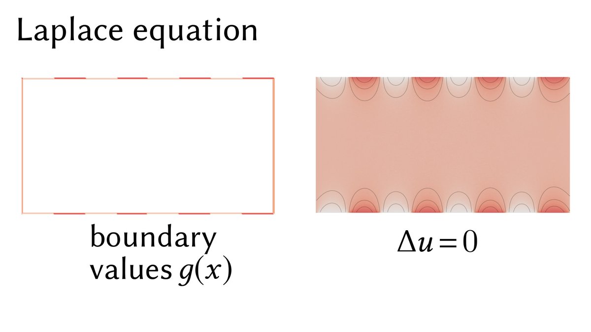
First, a Laplace equation Δu = 0 describes the steady-state temperature if heat is fixed to some function g on the boundary.

(Here the Laplacian Δ is just the sum of all 2nd partial derivatives: Δu = ∂²u/∂x² + ∂²u/∂y².)

[20/n]

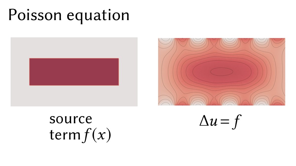
Adding a source term f yields a Poisson equation Δu = f, where f describes a "background temperature." Imagine heat being pumped into the domain at a rate f(x) for each point x of the domain.

[21/n]

We can control the rate of heat diffusion by replacing the Laplacian Δu, which can be written as ∇⋅∇u, with the operator ∇⋅(α∇ u), where the α(x) is a scalar function.

Physically, α(x) might describe, say, the thickness of a material, or varying material composition
[22/n]

Adding a drift term ω⋅∇ u to a Poisson equation indicates that heat is being pushed along some vector field ω(x) — imagine a flowing river, which mixes hot water into cold water until it reaches a steady state.

[23/n]

Finally, an absorption (or "screening") term σ(x)u acts like a background medium that absorbs heat—think about a heat sink, or a cold engine block. The function σ(x) describes the strength of absorption at each point x.

[24/n]

There are lots of other terms you could add to a PDE, but these already get you pretty far. And importantly, these are terms we'll be able to easily convert into integral & stochastic representations—and ultimately into Monte Carlo algorithms for PDEs! Let's see how…
[25/n]

Whereas a PDE described a function via derivatives, an integral equation uses, well, integrals!

A good example is deconvolution: given a blurry image f and a blur kernel K, can I solve

f(p)=∫ K(p,q) φ(q) dq

for the original image φ? [26/n]

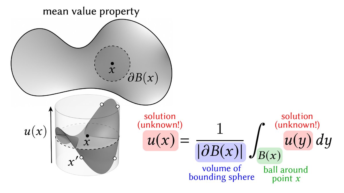
The solutions to basic PDEs can also be expressed via integral equations (IE). E.g., the solution to a Laplace equation is given by the so-called "mean value principle"

u(p)=∫_B(p) u(q) dq / |B(p)|

"The solution at p equals the average value over any ball B(p) around p" [27/n]

Unlike deconvolution, the IE for a Laplace equation is *recursive*: unknown values u(x) depend on unknown values u(y)!

Sounds like a conundrum, but this is *exactly* how modern rendering works: solve the recursive rendering equation by recursively estimating illumination. [28/n]

As with PDEs, we can keep adding terms to our IE to capture additional behavior (absorption, drift, ...).

For instance, there's a nice integral representation for a screened Poisson equation Δu−σu=−f, as long as absorption σ is constant in space! (See paper for details) [29/n]

Finally, we can describe the same phenomena using stochastic differential equations (SDE). For us, the stochastic picture is super important because it lets us deal with spatially-varying coefficients. We can then formulate an IE that can be estimated much as in rendering! [30/n]

An *ordinary* differential equation (ODE) describes the location X of a particle in terms of its derivatives in time. For instance, the ODE

dXₜ = ω(Xₜ) dt

says that the particle's velocity is given by some vector field ω—like a tiny speck of dust blowing in the wind.

[31/n]

A *stochastic* DE describes random motions—a key example is a Brownian motion Wₜ, where changes in position follow a Gaussian distribution, and are independent of past events.

Brownian motion describes everything from jiggling molecules to fluctuations in stock prices. [32/n]

Adding Brownian motion to our earlier ODE gives a more general *diffusion process*

dXₜ = ω(Xₜ) dt + dWₜ,

which we can think of as either a deterministic particle "with noise"—or as a random walk "with drift." Maybe something like dust blowing in hot, turbulent wind. [33/n]

We can also modulate the "strength of jiggling" via a function α(x), yielding the SDE

dXₜ = √α(Xₜ) dWₜ

As α increases, things sort of "heat up," and particles jiggle faster. [34/n]

Finally, we can think about a random walker that has some chance of getting absorbed in a background medium, like ink getting soaked up in a sponge.

We'll use σ(x) for the strength of absorption—which doesn't appear in the SDE itself, but will be incorporated in a moment. [35/n]

As you might have guessed, it's no coincidence that we use the same symbols α, σ, ω for both our PDE and our SDE!

These perspectives are linked by the infamous Feynman-Kac formula, which gives the solution to our main PDE as an expectation over many random walks.

[36/n]

A special case of Feynman-Kac that helps illustrate the idea is Kakutani's principle, which says the solution to a Laplace equation is the average value "seen" by a Brownian random walker when it first hits the boundary. See this thread for more:

https://twitter.com/keenanisalive/status/1258152691206893570

[37/n]

Most important for us: unlike classic (deterministic) integral equations, Feynman-Kac handles spatially-varying coefficients!

We can hence use it to build a *new* recursive-but-deterministic IE, which in turn leads to Monte Carlo methods for variable-coefficient PDEs. 🥵
[38/n]

To do so, we apply a "cascading" sequence of transformations to our original PDE to move all spatial variation to a (recursive!) to the right-hand side. This final PDE looks like a *constant*-coefficient screened Poisson equation, but with a (recursive!) source term. [39/n]

From the FEM perspective, it feels like we haven't done anything useful: we just shuffled all the hard stuff to the other side of the "=" sign. So what?

Yet from the Monte Carlo perspective we now have a way forward: recursively estimate the integral, a la path tracing!

[40/n]

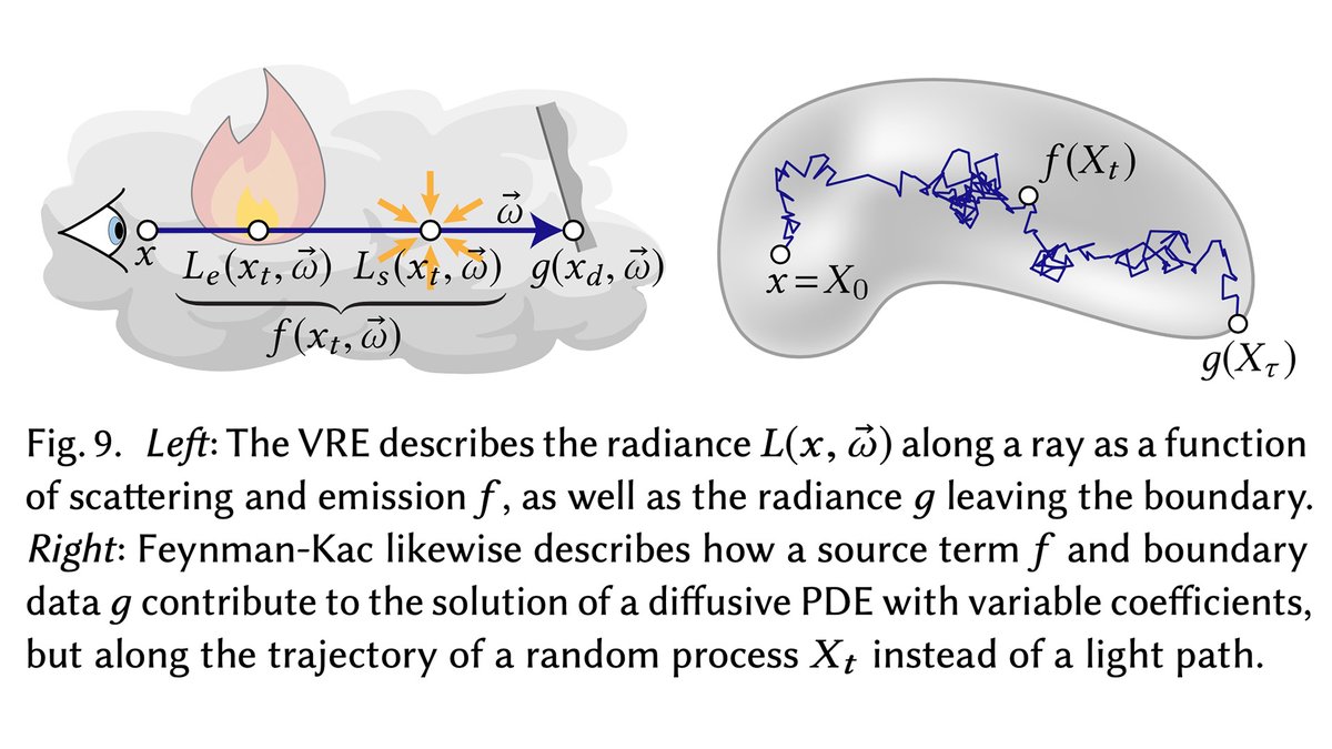
In fact, the relationship between PDEs and rendering is more than skin deep: the Feynman-Kac formula and the volumetric rendering equation (VRE) have an extremely similar form—which means we can adapt techniques from volume rendering to efficiently solve our PDE! [41/n]

This is really the moment of beauty, where PDEs suddenly benefit from decades of rendering research.

The paper describes how to apply delta tracking, next-flight estimation, and weight windows to get better estimators for PDEs. But *so* much more could be done here! [42/n]

Finally, you probably want to hear about applications.

Though our main goal here is to develop core knowledge, there are some cool things we can immediately do.

One is to simply solve physical PDEs with complex geometry, coefficients, etc., as in the "teaser" above. [43/n]

A graphics example is to generalize so-called "diffusion curves" to variable coefficients, giving more control over, e.g., how sharp or fuzzy details look.

(With constant-coefficient solvers, all the background details just get blurred out of existence!) [44/n]

Another nice point of view is that variable coefficients on a flat domain can actually be used to model constant coefficients on a curved domain! This way, we can solve PDEs with extremely intricate boundary data on smooth surfaces—without any meshing/tessellation at all. [45/n]

A Monte Carlo method also makes it easy to integrate PDE solvers with physically-based renderers. For instance, we can get a way more accurate diffusion approximation of heterogeneous subsurface scattering—without painfully hooking up to a FEM/grid-based solver. [46/n]

I've said way too much already, but the TL;DR is: grid-free Monte Carlo is a young and wicked cool way to solve PDEs, with deep-but-unexplored connections to rendering. It also still lacks some very basic features—like Neumann boundary conditions!

So, come help us explore! [n/n]