Thread by @ben_moll

Over the last decades, many asset valuations have gone through the roof. This had large effects on the distribution of wealth.

But what does it mean for welfare? Was this a huge shift of resources toward the wealthy? Or just welfare-irrelevant "paper gains"?

🧵 on a new paper:

The paper is joint work with @AndreasFagereng, Matthieu Gomez, Emilien Gouin-Bonenfant @BlomhoffHolm and @GNatvik

Paper here: benjaminmoll.com/APR/

Slides here: benjaminmoll.com/APR_slides/

In the economics debate, there are two opposing viewpoints:

On one hand, economists including @PikettyLeMonde @gabriel_zucman @dannyyagan & Saez have argued that wealth gains due to rising valuations are a big shift of resources toward the wealthy.

A frequent next step in the argument is that these should be taxed, e.g. by means of a wealth tax or a tax on unrealized capital gains.

See for example eml.berkeley.edu/~yagan/Capital… or @RonWyden's “Billionaires Income Tax” proposal finance.senate.gov/chairmans-news…

On the other hand, @JohnHCochrane @paulkrugman and others have argued that these wealth gains are just “paper gains”, with no effect on actual income flows and therefore welfare.

See for example johnhcochrane.blogspot.com/2020/01/wealth… and nytimes.com/2021/10/05/opi…

Which (if any) of these two opposing views is correct?

Who are the winners and losers of from rising asset valuations?

That's what this paper is about.

Our main contribution is a simple sufficient statistics formula for the money metric welfare gains/losses from asset price changes...

... which we then use to quantify these welfare gains/losses in Norway for the period 1994 to 2015.

The formula looks like this (in the special case of one asset) where
- i = individual
- T = sample period
- R = discount rate
- Sales_it = net sales of asset (Sales_it< 0 = purchase)
- Price Deviation_t = change in asset price relative to a baseline scenario

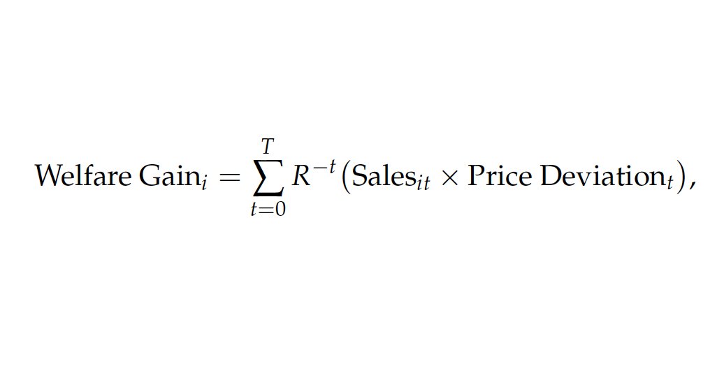
Importantly, the welfare gain is computed holding the asset's cash flows constant so that price deviations represent a pure valuation effect: a change in price without a change in cash flows.

In the data, we've seen a lot of this, eg due to the secular decline in interest rates.

"Money metric" here means welfare gains are in dollar terms. Like equivalent and compensating variation from intermediate micro (which are equivalent to 1st order)

The formula follows straight from an application of the envelope theorem and thus holds for small price deviations.

The welfare formula generates two main insights:

1. What matters are asset transactions not asset holdings.

Example: for someone who never sells an asset, rising asset prices are indeed just "paper gains".

But they *do* benefit prospective sellers and harm prospective buyers.

The most intuitive example is housing: skyrocketing house prices, say in London or Paris, benefit people who bought a house 30 years ago and now want to downsize, eg old people whose kids have moved out. But they hurt people who want to buy a house or upsize, eg young people.

2. Asset price changes are purely redistributive.

That's because they redistribute from buyers to sellers. But there's a buyer for every seller (once you include foreigners, the government etc).

Hence also our title "Asset-Price Redistribution"

With this in mind, let's come back to the two opposing viewpoints I mentioned above.

In a nutshell: both are incomplete and miss important parts of the equation.

Most of the intuition for our results can be seen in a simple two-period model. See section 1.2.

I particularly like a simple graphical intuition due to Whalley (1979). I've written about this paper before. Make sure to check it out. It's a gem.

https://twitter.com/ben_moll/status/1353773999566819329?s=20&t=QZX7lStOumMPjG0ybAKW8Q

People often ask: if I have an asset whose price increases so that market value of my wealth increases, how can that possibly be bad for me?

Answer: while the price increase raises your initial asset return, it *decreases* future returns. You're forgetting the second effect.

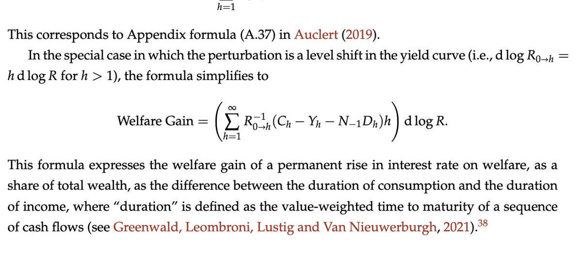
Note: our baseline formula abstracts from some important considerations, eg risk, bequests, rising asset prices loosening collateral constraints, people using "buy, borrow, die" strategies, wealth in utility, etc

Section 2.4 covers these extensions and shows how formula changes.

To implement our formula empirically we turn to Norway. Why Norway? Simply because they have 👌 data.

In particular: administrative panel data on all asset transactions over a 20 year time period. And remember: data on transactions is exactly what we need for our formula!

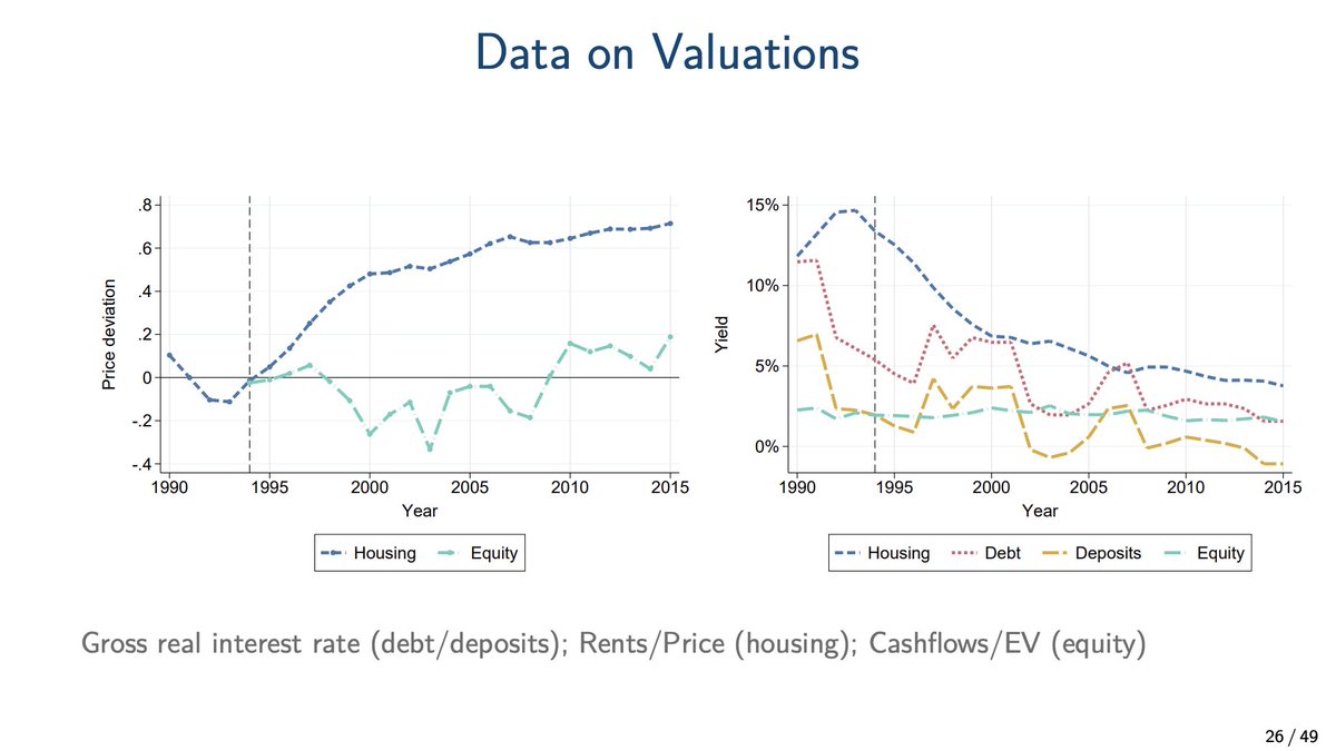
To isolate pure valuation effects, we compute price deviations as deviations from a baseline with prices growing at the same rate as dividend (or rents in the case of housing). For example here are Norwegian house prices, rents and the implied price deviations.

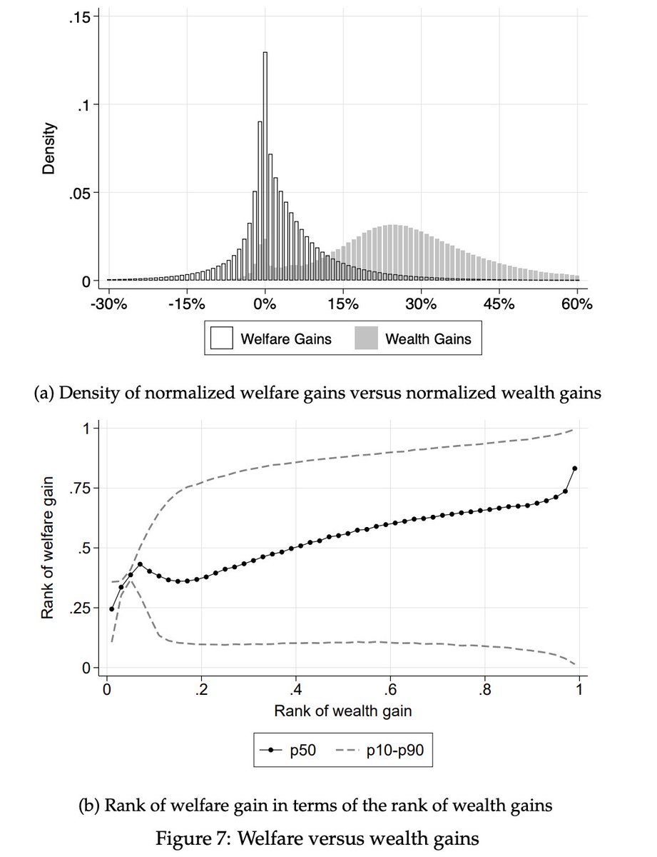
First main finding: rising asset prices have large redistributive effects.

Check out the histogram...

... which is even heavily truncated: the money metric welfare gain is −$280,000 at P1, about $1,000,000 at P99, and about $5,000,000 at P99.9 (i.e., for the top 0.1%).

As expected, the histogram is also centered around zero reflecting the redistributive nature of asset price changes.

Where do these large gains and losses come from? Answer: mostly housing and debt.

Importantly though: welfare gains differ substantially from naïvely calculated wealth gains (i.e. unrealized capital gains).

So does the identity of winners and losers implied by the two approaches. The two quantities are correlated but very far from equal.

Second main finding: large redistribution across cohorts, in particular from the young to the old.

That should be unsurprising given the important role for housing.

Interestingly, declining mortgage rates partly offset the welfare losses of the young due rising house prices.

Third main finding: large redistribution across the wealth distribution, from the poor to the wealthy.

Note that this isn't obvious: it comes from rich people
- selling houses
- holding lots of debt through private businesses and thus benefiting from low interest rates

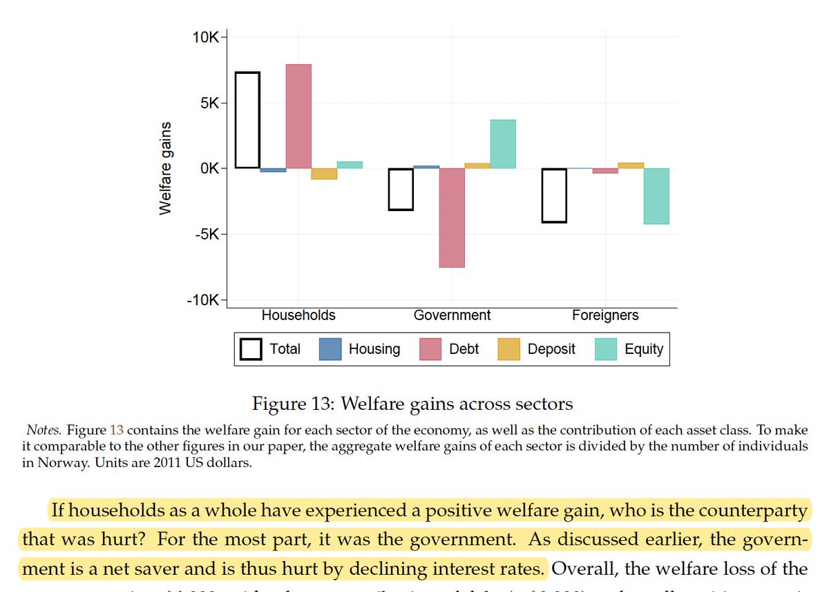
Fourth main finding: some redistribution across sectors. Declining interest rates benefited households at the expense of the government.

Note that the Norwegian case is a bit unusual here, partly because of the large sovereign wealth fund. We still need to dig deeper here.

Our findings build on a large literature, including some classics.

For instance, I highly recommend the very lucid discussion of related issues in Kaldor's 1955 book "An Expenditure Tax", see benjaminmoll.com/kaldor/. As well as the Whalley paper I already mentioned.

More recently, and probably most related, important work by @ProfGreenwald @matteoleombroni @HannoLustig and @SVNieuwerburgh.

See this great thread by @HannoLustig:

https://twitter.com/HannoLustig/status/1445720253242040320?s=20&t=yaKCBtHhSgJ0eYk8api8rg

The connection between the two papers is explained in Section 2.4.

And finally important work on wealth inequality and asset prices by @cmtneztt @kuhnmo @MSchularick @omzidar @sc_cath @ric_cioffi and many others.

Also related: @mdoepke and Schneider on the redistributive effects of inflation and @andyecon @Jonheathcote @DirkKrueger7.

In summary: asset price changes have large redistributive effects.

But it's a bit subtler than just: those who own assets become wealthier and therefore win.

Let me conclude with a question: what does this mean for optimal taxation? Some speculative thoughts below.

But to do this properly we need to finally put the "finance" into "public finance" in the sense of studying optimal taxation in environments with changing asset prices!

In case I managed to wet your appetite, also make sure to tune in tomorrow for my coauthor Emilien presenting in @glviolante @GregWKaplan and Hurst's group, also on the @nberpubs YouTube channel youtube.com/nbervideos

nber.org/conferences/si…