Post

How to get URL link on X (Twitter) App

On the Twitter thread, click on or icon on the bottom
Click again on or Share Via icon
Click on Copy Link to Tweet
Paste it above and click "Unroll Thread"!
More info at Twitter Help

Peyman Milanfar

@docmilanfar

Oct 7, 2022 • 8 tweets • 8 min read • Read on X

Scrolly

@GooglePhotos

Today we announced a new feature on Pixel 7/Pro and @GooglePhotos called "Unblur". It's the culmination of a year of intense work by our amazing teams. Here's a short thread about it

1/n

#MadeByGoogle #fixedonpixel #Pixel7 #PhotoUnblur
@GooglePixel_US

Last yr we brought two new editor functions to Google Photos: Denoise & Sharpen. These could improve the quality of most images that are mildly degraded. With Photo Unblur we raise the stakes in 2 ways:

First, we address blur & noise together w/ a single touch of a button.

2/n

Second, we're addressing much more challenging scenarios where degradations are not so mild. For any photo, new or old, captured on any camera, Photo Unblur identifies and removes significant motion blur, noise, compression artifacts, and mild out-of-focus blur.

3/n

Photo Unblur works to improve the quality of the 𝘄𝗵𝗼𝗹𝗲 photo. And if faces are present in the photo, we make additional, more specific, improvements to faces on top of the whole-image enhancement.

4/n

One of the fun things about Photo Unblur is that you can go back to your older pictures that may have been captured on legacy cameras or older mobile devices, or even scanned from film, and bring them back to life.

5/n

It's also fun to go way back in time (like the 70s and 80s !) and enhance some iconic images like these photos of pioneering computer scientist Margaret Hamilton, and basketball legend Bill Russell.

6/n

@2ptmvd

Recovery from blur & noise is a complex & long-standing problem in computational imaging. With Photo Unblur, we're bringing a practical, easy-to-use solution to a challenging technical problem; right to the palm of your hand
w/ @2ptmvd @navinsarmaphoto @sebarod & many others

n/n

Bonus: Once you have a picture enhanced with #PhotoUnblur, applying other effects on top can have an even more dramatic effect. For instance, here I've also blurred the background and tweaked some color and contrast.

• • •

Missing some Tweet in this thread? You can try to force a refresh

This Thread may be Removed Anytime!

Twitter may remove this content at anytime! Save it as PDF for later use!

More from @docmilanfar

Peyman Milanfar

@docmilanfar

Nov 10

Integral geometry is a beautiful topic bridging geometry, probability & statistics

Say you have a curve with any shape, possibly even self-intersecting. How can you measure its length?

This has many applications - curve could be a strand of DNA or a twisted length of wire

1/n

A curve is a collection of tiny segments. Measure each segment & sum. You can go further: make the segments so small they are essentially points, count the red points

A practical way to do this: drop many lines, or a dense grid, intersecting the shape & count intersections

2/n

Curve's length is the sum of intersections n(ρ,θ) of all lines (in polar coords) with the curve (counting multiplicities). This is the beautiful Crofton formula:

Length = 1/2 ∫∫ n(ψ,p) dψ dp

The 1/2 is there because oriented lines are a double cover of un-oriented lines

3/n

Read 6 tweets

Peyman Milanfar

@docmilanfar

Sep 24

Smoothing splines fit function to data as the sol'n of a regularized least-squares optimization problem.

But it’s also possible to do it in one shot with an unusually shaped kernel (see figure)

Is it possible to solve other optimization problems this way? Surprisingly yes

1/n

This is just one instance of how one can “kernelize” an optimization problem. That is, approximate the solution of an optimization problem in just one-step by constructing and applying a kernel once to the input

Given some conditions you can it do much more generally

2/n

If you specialize the regularization to be of the form
φ(x) = ρ( ||Ax|| ) where A= R(|i-j|) is a stationary & isotropic, this gives tidy conversions between φ(x) and the kernel K(x).

3/n

Read 4 tweets

Peyman Milanfar

@docmilanfar

Sep 18

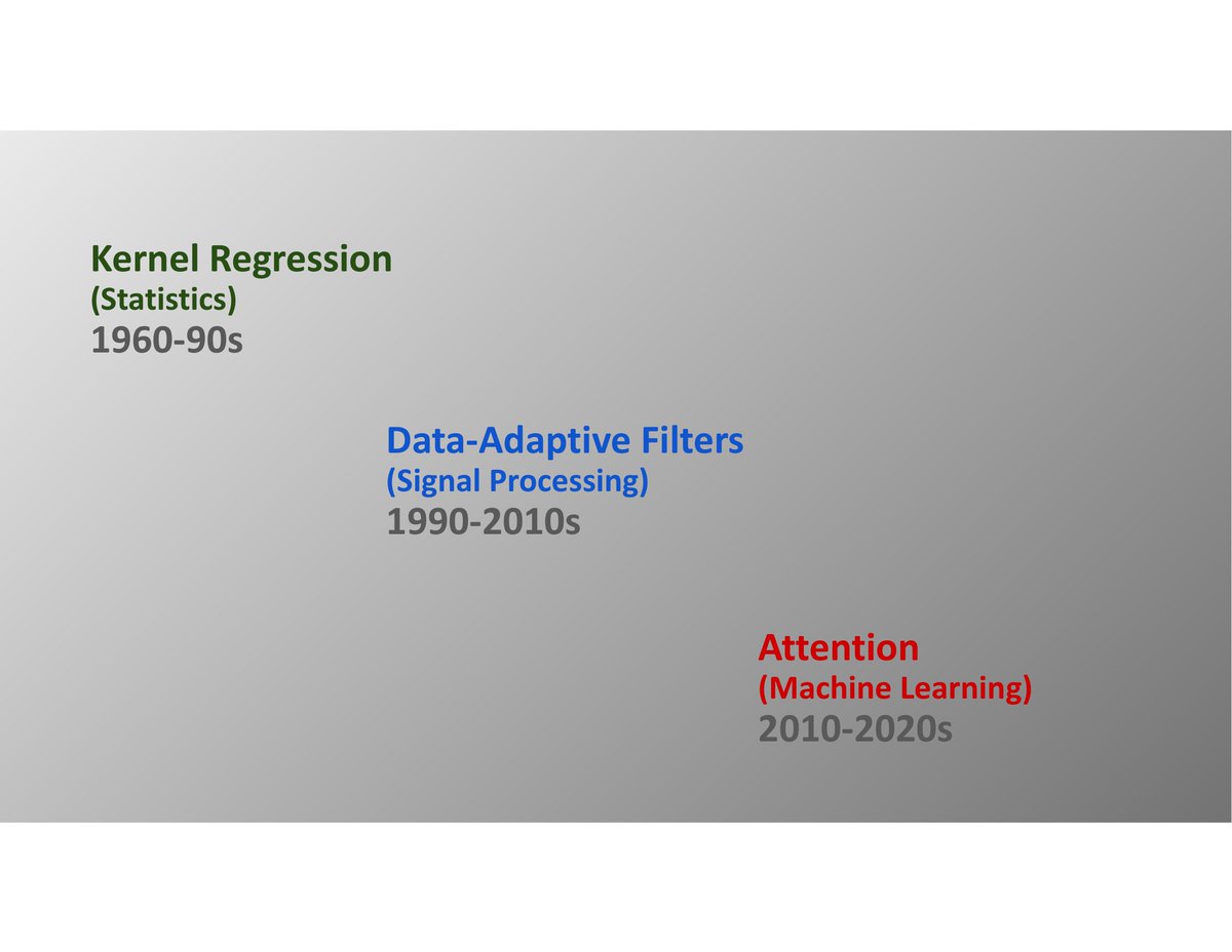
Mean-shift iteratively moves points towards regions of higher density. It does so by placing a kernel at each data point, calculating the mean of the data points within that window, shifting points towards this mean until convergence: Look familiar?

1/n
(Animation @gabrielpeyre)

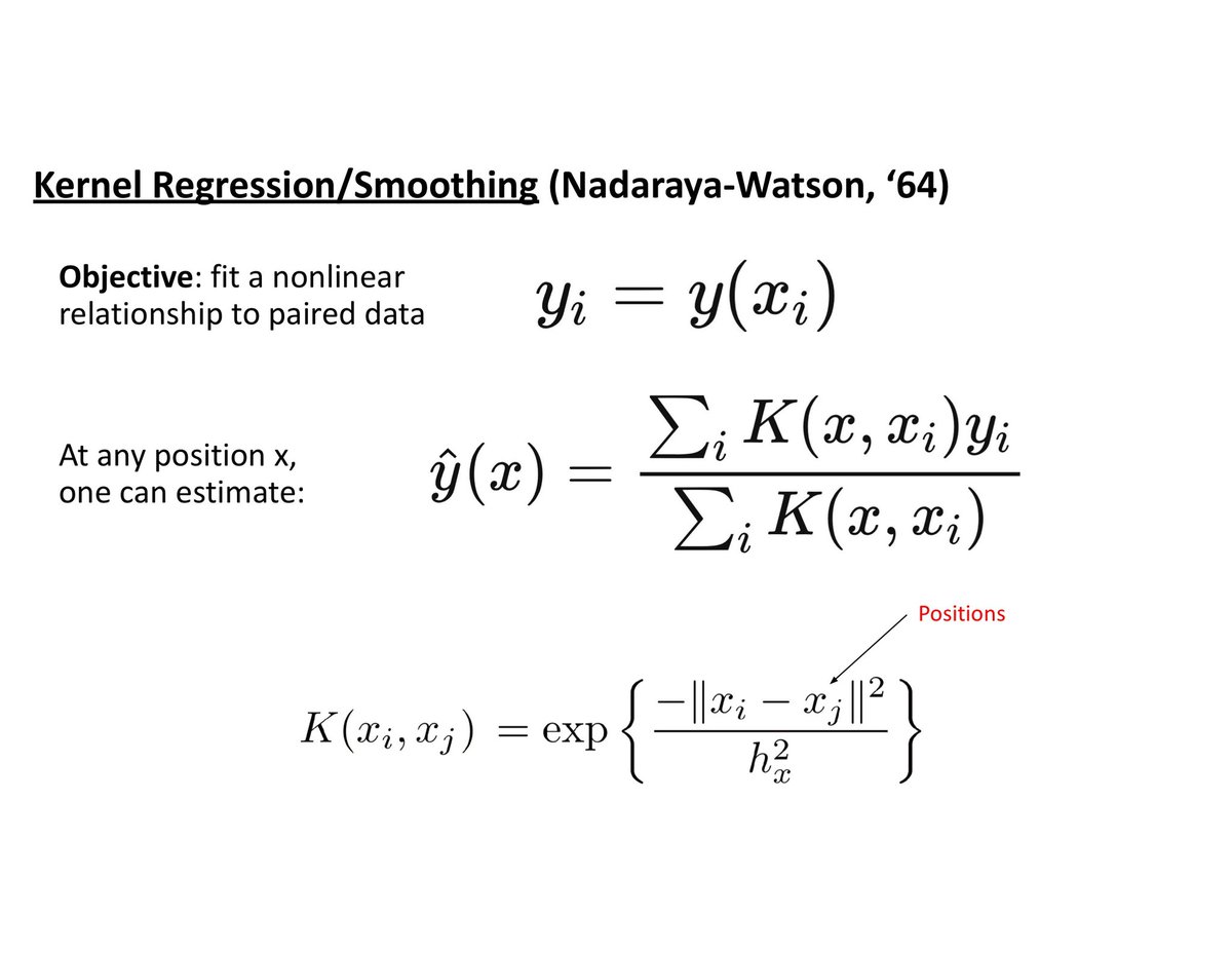
The first term on the right hand side of the ODE has the form of a pseudo-linear denoiser f(x) = W(x) x. A weighted average of the points where the weights depend on the data. The overall mean-shift process is a lot like a residual flow:

d/dt x(t) = f(x(t)) - x(t)

2/n

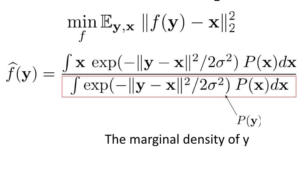
Residual on the RHS is an approximation of the “score” -the gradient of the empirical density of x making it a gradient flow

d/dt x(t) ≈ ∇ log p̂(x(t))

So mean-shift a) estimates the empirical density & b) flows points to nearby peaks. Similarly to flow-matching & InDI

3/n

Read 4 tweets

Peyman Milanfar

@docmilanfar

Sep 5

Random matrices are very important in modern statistics and machine learning, not to mention physics

A model about which much less is known is uniformly sampled matrices from the set of doubly stochastic matrices: Uniformly Distributed Stochastic Matrices

A thread -

1/n

First, what are doubly stochastic matrices?
Non-negative matrices whose row & column sums=1.

The set of doubly stochastic matrices is also known as the Birkhoff polytope: an (n−1)² dimensional convex polytope in ℝⁿˣⁿ with extreme points being permutation matrices.

2/n

The extreme points of the Birkhoff polytope (permutations) are sparse matrices, but a typical matrix sampled from inside the polytope is by contrast, very dense

Since rows and columns are exchangeable, the entries of a sampled matrix have the same marginal distribution.

3/n

Read 8 tweets

Peyman Milanfar

@docmilanfar

Sep 1

The perpetually undervalued least-squares:

minₓ‖y−Ax‖²

can teach a lot about some complex ideas in modern machine learning including overfitting & double-descent.

Let's assume A is n-by-p. So we have n data points and p parameters

1/10

If n ≥ p (“under-fitting” or “over-determined" case) the solution is

x̃ = (AᵀA)⁻¹ Aᵀ y

But if n < p (“over-fitting” or “under-determined” case), there are infinitely many solutions that give *zero* training error. We pick min‖x‖² norm solution:

x̃ = Aᵀ(AAᵀ)⁻¹ y

2/10

In either case, the solution can be compactly written in terms of the SVD of A:

A = USVᵀ

where U & V are orthogonal matrices of size nxn & pxp, and S is nxp & contains i = 1 to k nonzero diag elements

x̃ = ∑ σᵢ⁻¹ vᵢ uᵢᵀ

where σᵢ are the nonzero sing vals of S

3/10

Read 10 tweets

Peyman Milanfar

@docmilanfar

Aug 18

Two basic concepts are often conflated:

Sample Standard Deviation (SD) vs Standard Err (SE)

Say you want to estimate m=𝔼(x) from N independent samples xᵢ. A typical choice is the average or "sample" mean m̂

But how stable is this? That's what Standard Error tells you:

1/6

Since m̂ is itself a random variable, we need to quantify the uncertainty around it too: this is what the Standard Error does.

The Standard Error is *not* the same as the spread of the samples - that's the Standard Deviation (SD) - but the two are closely related:

2/6

But this expression isn't practical because we don't know √var(xᵢ) either

Not knowing √var(xᵢ), we are forced to estimate that too. Here, we typically just plug in the (sample) Standard Deviation for it. Therefore:

Standard Error ≈ Sample Standard Deviation/√N

3/6

Read 7 tweets

Support us! We are indie developers!

This site is made by just two indie developers on a laptop doing marketing, support and development! Read more about the story.

Become a Premium Member ($3/month or $30/year) and get exclusive features!

Become Premium

Don't want to be a Premium member but still want to support us?

Make a small donation by buying us coffee ($5) or help with server cost ($10)

Donate via Paypal

Or Donate anonymously using crypto!

Ethereum

0xfe58350B80634f60Fa6Dc149a72b4DFbc17D341E copy

Bitcoin

3ATGMxNzCUFzxpMCHL5sWSt4DVtS8UqXpi copy

Thank you for your support!

Share this page!

Enter URL or ID to Unroll

Peyman Milanfar

Try unrolling a thread yourself!

More from @docmilanfar

Peyman Milanfar

Peyman Milanfar

Peyman Milanfar

Peyman Milanfar

Peyman Milanfar

Peyman Milanfar

Did Thread Reader help you today?

Don't want to be a Premium member but still want to support us?

Send Email!