Thread by @TivadarDanka

The single most undervalued fact of linear algebra: matrices are graphs, and graphs are matrices.

Encoding matrices as graphs is a cheat code, making complex behavior simple to study.

Let me show you how!

If you looked at the example above, you probably figured out the rule.

Each row is a node, and each element represents a directed and weighted edge. Edges of zero elements are omitted.

The element in the 𝑖-th row and 𝑗-th column corresponds to an edge going from 𝑖 to 𝑗.

To unwrap the definition a bit, let's check the first row, which corresponds to the edges outgoing from the first node.

Similarly, the first column corresponds to the edges incoming to the first node.

Here is the full picture, with the nodes explicitly labeled.

Why is the directed graph representation beneficial for us?

For one, the powers of the matrix correspond to walks in the graph.

Take a look at the elements of the square matrix. All possible 2-step walks are accounted for in the sum defining the elements of A².

If the directed graph represents the states of a Markov chain, the square of its transition probability matrix essentially shows the probability of the chain having some state after two steps.

There is much more to this connection.

For instance, it gives us a deep insight into the structure of nonnegative matrices.

To see what graphs show about matrices, let's talk about the concept of strongly connected components.

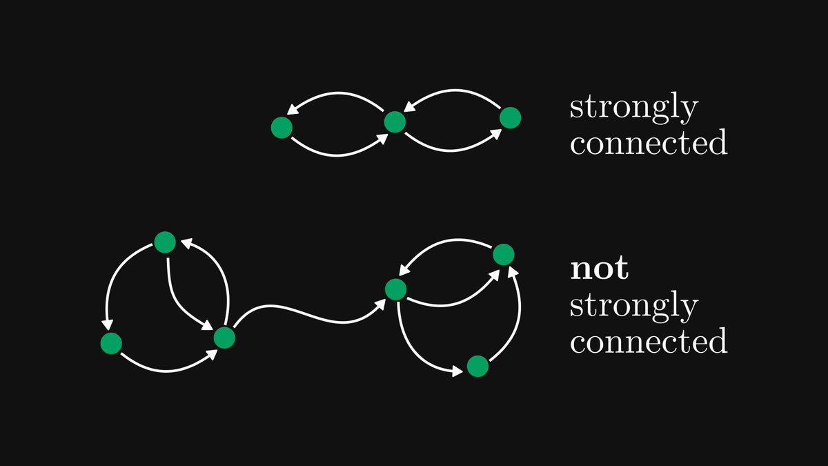
A directed graph is strongly connected if every node can be reached from every other node.

If this is not true, the graph is not strongly connected.

Below, you can see an example of both.

Matrices that correspond to strongly connected graphs are called irreducible. All other nonnegative matrices are called reducible. Soon, we'll see why.

(For simplicity, I assumed each edge to have a unit weight, but each weight can be an arbitrary nonnegative number.)

Back to the general case!

Even though not all directed graphs are strongly connected, we can partition the nodes into strongly connected components.

Let's label the nodes of this graph and construct the corresponding matrix!

(For simplicity, assume that all edges have unit weight.)

Do you notice a pattern?

The corresponding matrix of our graph can be reduced to a simpler form!

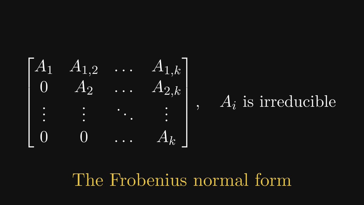
Its diagonal comprises blocks whose graphs are strongly connected. (That is, the blocks are irreducible.) Furthermore, the block below the diagonal is zero.

In general, this block-matrix structure is called the Frobenius normal form.

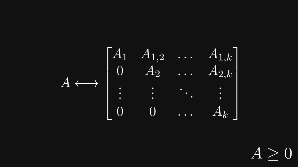
Let's reverse the question: can we transform an arbitrary nonnegative matrix into the Frobenius normal form?

Yes, and with the help of directed graphs, this is much easier to show than purely using algebra.

This is just the tip of the iceberg. For example, with the help of matrices, we can define the eigenvalues of graphs!

Utilizing the relation between matrices and graphs has been extremely profitable for both graph theory and linear algebra.

To sum it all up, this was the haiku I wrote when I first discovered the connection between graphs and matrices:

"To study structure,
tear away the flesh, until
only the bone shows."

This thread is just ~30% of the full post, which you can find on my Substack. It is filled with exciting stuff, so check it out: thepalindrome.substack.com/p/matrices-and…

If you have enjoyed this thread, follow me, and subscribe to my newsletter!

Mathematics is fantastic, and I regularly post deep-dive explanations about seemingly complex concepts from mathematics and machine learning.

thepalindrome.substack.com