Thread by @keenanisalive

[1/n] There's been a lot of hubbub lately about the best known packing of 17 unit squares into a larger square, owing to this post:

https://twitter.com/KangarooPhysics/status/1625423951156375553

I realized this can be coded up in < 5 minutes in the browser via @UsePenrose, and gave it a try. Pretty darn close! 🧵

[2/n] To be clear, this 🧵 isn't about finding a better packing—or even finding it faster. Wizards like @KangarooPhysics surely have better tricks up their sleeves 🪄

Instead, it's about an awesome *tool* for quickly whipping up constraint-based graphics: penrose.cs.cmu.edu

[3/n] The "17 squares" problem provides a great demonstration of how Penrose works.

In fact, if you want to use this thread as a mini-tutorial, you can try it out at penrose.cs.cmu.edu/try/

[4/n] The first step is to just say what type of objects we have in our domain of interest.

In this case, there's just one type of object: squares!

So, we write "type Square" in the domain tab:

[5/n] Next, we need to say how squares should get "styled," i.e., how they should get arranged and drawn. So, let's open up the style tab:

[6/n] The first thing is to just say how large our drawing canvas should be.

Since the drawing will be forced to stay on the canvas, we can use the canvas itself as the outer bounding square!

The smaller we make the width/height, the harder packing our 17 squares will become…

[6/n] The first thing is to just say how large our drawing canvas should be.

Since the drawing will be forced to stay on the canvas, we can use the canvas itself as the outer bounding square!

The smaller we make the width/height, the harder packing our 17 squares will become…

[7/n] Next up: how should we draw each Square?

Well, we can make a rule for that: for all squares, draw a polygon with four corners, centered around the origin.

[8/n] So far we've said that we want to draw squares, and have specified how to draw a square.

But to see something actually pop up on the screen, we have to actually make a square!

So, let's head over to the "substance" tab and just type "Square S".

[9/n] Hit "compile" and you should now see a lonely square.

…not that exciting!

But it's gonna get way more interesting really fast.

[10/n] Let's hop back over to the style tab, where all the action happens.

First, we'll give our square a variable translation (x,y) and rotation θ, using some standard 2D vector math.

The ? mark means Penrose will fill in the blanks for us (e.g., by picking random values).

[11/n] If we hit "compile▸" again, we now get a random square fitting this description.

Hit "resample", and we get a different random square.

Notice that the square always stays within the canvas—which will be essential for our packing problem!

[12/n] Finally—and this is really where the magic happens—we just tell Penrose that we don't want any squares to overlap.

In particular, for all pairs of distinct squares S and T, we ask that their "icons" (the shapes we defined in the previous rule) should be disjoint.

[13/n] Of course, since we only asked for one square, this rule is gonna be really easy to satisfy!

So, let's go back to the "substance" tab and this time ask for all seventeen:

[14/n] If we now hit "compile", we should see something that looks like confetti—because our bounding box is super huge (100 x 100):

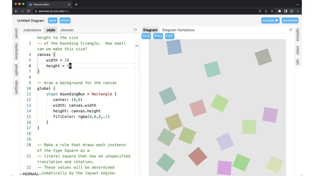
[15/n] But what if we try a smaller box, say, 10 x 10 (by changing the canvas size at the top of the "style" program)?

More interesting…

[16/n] Maybe to see what's going on we should draw a background for the canvas:

[17/n] Now we can make the bounding box 5x5…

[18/n] 4.8 x 4.8…

[19/n] And keep on going—how low can we go?

Warning: if you make it too small, the optimization may go on forever and freeze your tab! Sorry about that.

You can also slow down the optimization to a step size of 1 to see how it works:

From here of course you can pack a different number of squares, or different shapes altogether.

But really this is just a (very) small example of what you can do with Penrose—check out the gallery and documentation for more.

And have fun exploring!

[20/20]

P.S. Here's the full example if you don't feel like typing it in yourself!

penrose.cs.cmu.edu/try/?gist=b560…

Thread continues here:

https://twitter.com/keenanisalive/status/1626707771294113792?s=20

(Not sure why it broke!)