One Iranian ingenuity that catch my attention. The Fateh-110 Ballistic missile. It looks simple, practical and appears to be good enough Tactical ballistic missile.
let's cut to the chase, the estimates are done in 13 frequencies from VHF down to X-band, i would love doing 35 frequencies as usual but i just dont want to wait 8 hours for it to complete. The missile is usual PEC as it's a metalic airframe.
In case someone interested with separate vids. This one depicts the half sphere contour plot
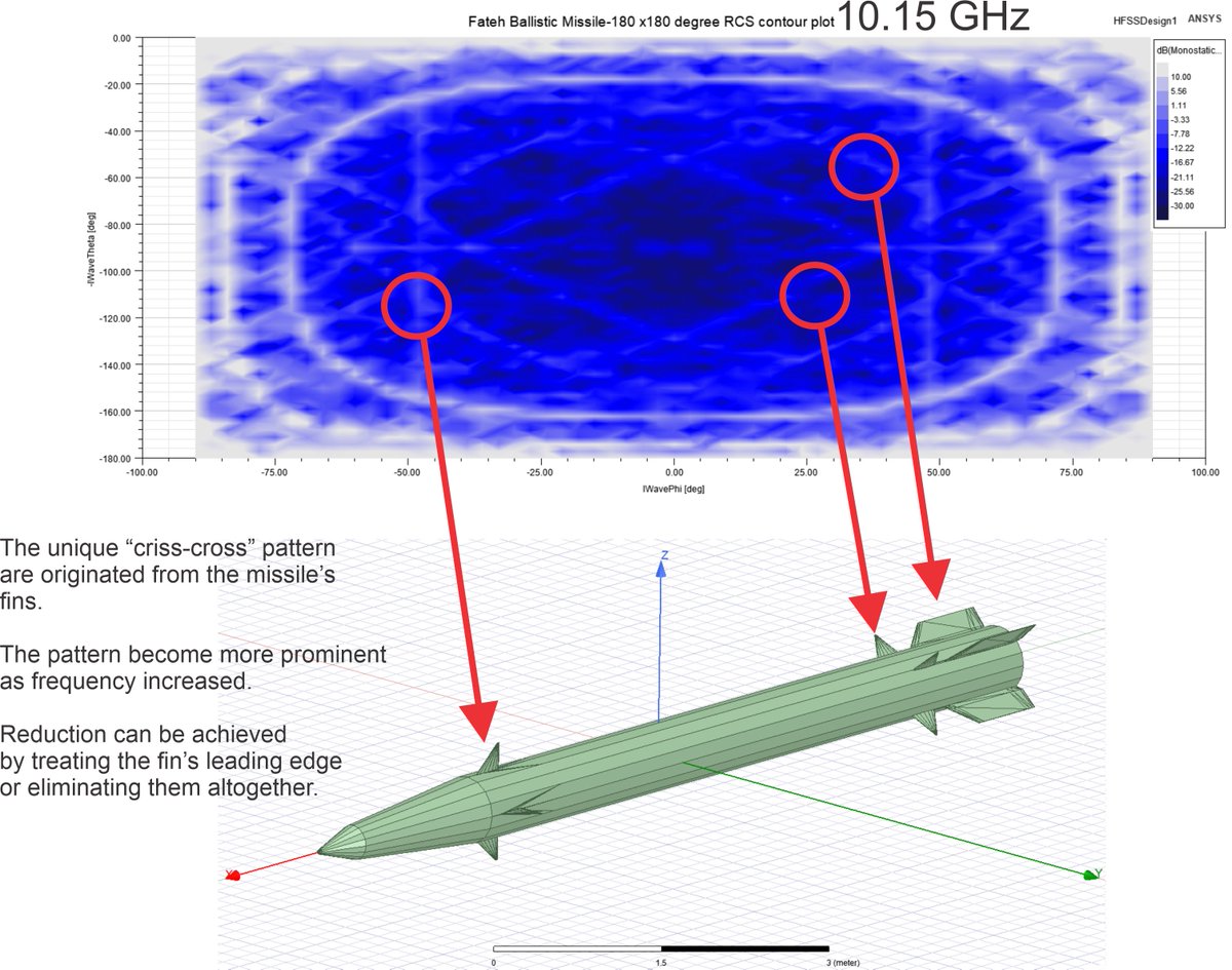
This one is the contour plot. in flat form. This one might look pretty for a praying mats.
And now some numbers. the medianized RCS value of the missile vs frequencies. Unfortunately i havent been able to properly fit the data into a model (e.g Swerling) so cant provide PDF (Probability Density Value) of the RCS.
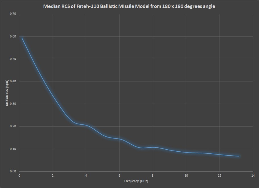
The PDF is important as it allows estimate of the likelihood of encountering specific RCS and therefore detectability of the target. Median is good but it only for limited angle.
The other presentation i havent able to provide was to give a time vs RCS value which more valuable as it takes account of the movement of the missile. ABM radar may detect the large side-aspect RCS of the Fateh as it breaks the horizon.
The contour plot tho reveal something nifty. namely the unique pattern produced by the missile's fins. these lobes are strong but narrow, so could be hard to pick. However if desired treatment is possible.
Guess that's all for now, back to other things. Anyway i'm always accepts commission for this kind of RCS visualizations. Also i can always use some support. as these kind of content does require processing power.
So more into the X-mas tree fighter of mine. First thing first that.. it's big a Flanker sized article. with 22 m length and also 22 m wingspan
Two iterations, one with RAM and another is not. To see what the basic shape can provide. and of course see if the RAM actually a good match. The treatement encompass the fuselage and wings. radome are left as PEC to approximate effect of bandpass radome.
Result is i would say satisfactory. As 62% reduction of RCS from RAM treatment is achievable across all simulated frequency. I also provide breakdown on "low" (VHF-L) and "high" (L to X) For clarity.
There are many forms of Radar Range Equation. Including one that you can use to calculate the amount of targets your radar can track.
The equation below show the relationship between Power aperture product/PAG and "radar resources" like -
The update time (basically your beam dwell time if your radar is a fulltime tracking) and the monopulse slope constant, a design dependent but usually taken as 1.2-1.6.
The equation favors High frequency radar, once frequency is selected tho.
The radar tracking performance will depend on its Power aperture product. Which in turn.. bigger radar do better than smaller one. Want more targets to track ? Get moar power or get bigger antenna or both if you AESA as your PAG scales with a power of 3 of your TRM numbers.
Schematics of Virupaksha radar for Indian "Super Sukhoi" Program. Including the TRM's. 30% less than what i estimated back then assuming Uttam's Frequency are used but still massive 2208 TRM's.
Assuming Bars sized (1 m diameter or 0.78 sqm area) The 2208 element counts and as seen Triangular lattice topology in element placements, assuming 120 degrees scan angle (+-60) will put the frequency in 9196 MHz. Close to Bars and my estimates on J-16 Radar.
That and assume 35% PAE (Power Added Efficiency) for the TRM (typical for class A-Amplifier type) The 10.5 KW cooling available from new VCM cooling Allows 6.6 KW Average power, an increase over 5 KW for Irbis-E. TRM peak power rating will depend on required-
As for the modeling. it's as usual "standard" of mine 120 x 45 degrees. The model is pure PEC and based on the 10 ft scale model tested for RCS by lockheed. The frequency is from VHF down to Ka Band (150 MHz down to 35 GHz)
So what if i take the canard away from a J-20 ? Will the RCS got smaller somehow ?
A simple comparison, between both model is done. They're mostly PEC and having same treatment. The purpose is to see what kind of RCS "reduction" coming from removing the canard.
The following is the 2D contour plot presentation for both subjects. 2D contour plot is basically same as the "porcupine" like 3D presentation i do except flattened into diagram and be given clearer angle.
This equation is your friend and will fight for your sanity.
This version of breguet range equation however assume constant L/D, Velocity and Isp. means it's good for a constant altitude and speed scenario.
Isp or Specific impulse are the measure of efficiency of a propulsion. It is the "inverse" of SFC (Specific Fuel Consumption). To convert one to the other you can divide 3600 with SFC. SFC for typical propulsions can easily be found online.