Number Needed to Treat (NNT) & Number Needed to Harm (NNH) in Clinical Trials Explained in Plain English 📊🩺
1/ When evaluating a new treatment, two key numbers often come up: Number Needed to Treat (NNT) and Number Needed to Harm (NNH). Let's demystify these in simple terms.
2/ 🎯 Number Needed to Treat (NNT):
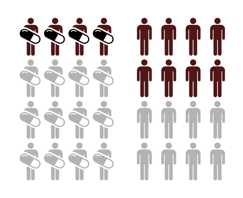
Imagine 100 people with a headache. If 80 get better with a new pill and 70 get better without it, then 10 benefitted from the pill. So, you'd need to treat 10 people for 1 to benefit. That's an NNT of 10.
3/ A lower NNT is generally better. If a drug has an NNT of 2, it means for every 2 people treated, 1 benefits. If it's 50, you'd have to treat 50 people for 1 to see a benefit. The smaller the number, the more effective the treatment.
4/ 🔥 Number Needed to Harm (NNH):
Now, let's say out of 100 people, 5 have a side effect from the pill. That means, for every 20 people treated, 1 person experiences harm. That's an NNH of 20.
5/ A higher NNH is preferred. If a drug has an NNH of 100, it means 1 out of 100 people treated might experience harm. If it's 10, then 1 out of every 10 might be harmed. The bigger the number, the safer the treatment (in terms of that specific harm).
6/ It's a balance! Healthcare professionals look at both NNT and NNH to decide if a treatment's benefits outweigh the risks. A drug might have an NNT of 5 (good) but an NNH of 6 (risky). So, while it's effective, there's also a notable risk.
7/ Real-world example: Aspirin can be recommended to prevent heart attacks. The NNT tells us how many need to take it to prevent one heart attack. But it can also cause bleeding, so the NNH tells us how many might take it before one person is harmed.
8/ When hearing about a new treatment, asking about NNT & NNH can give you a clearer picture. It's not just about "Does it work?" but also "How often does it work?" and "What's the risk?"
9/ In conclusion, NNT & NNH are tools to help understand the impact of treatments. They help us make informed choices, balancing benefits against potential harms.
10/ So next time you're discussing treatments, remember these numbers. They help simplify complex decisions, bringing clarity to the choices we make in healthcare.
If you found this post useful, please give it a ❤️ or 🔁. Sharing knowledge empowers everyone to make informed health decisions. Stay curious!
#DataScience #Statistics
• • •
Missing some Tweet in this thread? You can try to
force a refresh
1/10 High predictive performance in biological datasets (e.g., AUC > 0.95) should raise suspicion, not applause.
Is the signal real, or is it a batch effect?
The R/tidymodels ecosystem lacks standardized post-hoc tools to audit this.
Introducing bioLeak. 🧵 #rstats
2/10 We developed bioLeak to address a specific gap: the lack of systematic, post-hoc integrity checks for R-based machine learning.
It acts as an auditing layer for tidymodels objects, enabling methodological validation without altering existing training pipelines.
3/10 It uses label permutation to construct an empirical null distribution of the performance metric.
If the model performs well on shuffled labels, it shows the model is exploiting structural artifacts rather than biological signal.
A low "Permutation Gap" suggests invalidity.
In statistics and probability theory, a sample space is the set of all possible outcomes of a random experiment. It provides a comprehensive framework for understanding all potential results that could occur in a given scenario. The sample space is typically denoted by the symbol S.
#Statistics #DataScience #Research #Science
Examples:
1. Coin Toss: When flipping a fair coin, the sample space consists of two possible outcomes: heads (H) and tails (T). Thus, the sample space can be represented as:
S ={ H, T}
2. Rolling a Six-Sided Die: For a single roll of a standard six-sided die, the sample space includes all six possible outcomes:
S = i{ 1, 2, 3, 4, 5, 6}
3. Tossing Two Coins: When tossing two coins simultaneously, the sample space comprises all possible pairs of outcomes:
S ={ (H, H), (H, T), (T, H), (T, T)}
Importance in Probability:
Defining the sample space is a fundamental step in probability theory because it allows for the calculation of probabilities of various events. An event is any subset of the sample space, including single outcomes or groups of outcomes. For instance, in the die-rolling example, the event of rolling an even number is the subset { 2, 4, 6} .
The wisdom of crowds is a phenomenon where the collective judgment or estimate of a group can be remarkably accurate, often surpassing individual expertise. This principle is grounded in the idea that individual errors tend to cancel each other out when aggregated, provided the crowd is diverse, independent, and sufficiently large.
David Spiegelhalter’s jellybean experiment illustrates this concept vividly and highlights its statistical underpinnings.
1. The Experiment
• Spiegelhalter and James Grime conducted a simple yet revealing test of crowd intelligence. They posted a YouTube video displaying a jar of jellybeans and asked viewers to guess how many beans were inside.
• A total of 915 guesses were collected, ranging from 219 to an absurd 31,337.
2. Key Results
• The actual number of jellybeans in the jar: 1,616.
• The median guess (1,775) overestimated the true count by just 159 (10% error).
• The mean guess (2,408) was significantly less accurate due to the influence of extreme outliers, such as the guess of 31,337.
• Remarkably, the median guess was closer to the actual value than 90% of individual guesses.
In statistical modeling, particularly within the context of regression analysis and analysis of variance (ANOVA), fixed effects and random effects are two fundamental concepts that describe different types of variables or factors in a model. Here’s a straightforward explanation:
#Statistics #DataScience #Research #Science
Fixed Effects:
Fixed effects refer to variables or factors whose levels are specifically chosen and are of primary interest in the study. These effects are considered constant and non-random, meaning the conclusions drawn from them are applicable only to the specific levels included in the analysis.
Imagine you’re studying the impact of different teaching methods on student performance. If you specifically choose and focus on three methods—lecture, discussion, and online learning—these are your fixed effects. You’re interested in understanding how each of these particular methods affects performance, and your conclusions will apply only to these methods.
Random Effects:
Random effects pertain to variables or factors whose levels are randomly sampled from a larger population, and the interest extends beyond the specific levels included in the study. These effects are considered random variables, and the conclusions drawn can be generalized to the broader population from which the samples were taken.
Consider you’re evaluating the same teaching methods but across various schools. If you randomly select a few schools from a larger pool to include in your study, the ‘school’ factor becomes a random effect. Here, you’re not just interested in the specific schools chosen but aim to generalize your findings to all schools. The selected schools represent a random sample from the broader population, allowing your conclusions to extend beyond the sampled group.
Heteroscedasticity refers to a condition in regression analysis where the variance of the error terms, or residuals, is not constant across all levels of the independent variables. In other words, the spread of the residuals changes systematically with the values of the predictors. This violates the assumption of homoscedasticity, which states that residuals should have constant variance.
#Statistics #DataScience #Research #Science
Implications of Heteroscedasticity in Regression Analysis
1. Inefficiency of OLS Estimates: While ordinary least squares (OLS) estimators remain unbiased in the presence of heteroscedasticity, they are no longer efficient. This inefficiency means that OLS estimators do not achieve the minimum variance among all unbiased estimators, leading to less precise coefficient estimates.
2. Biased Standard Errors: Heteroscedasticity causes the estimated variances of the regression coefficients to be biased, leading to unreliable hypothesis testing. The t-statistics may appear more significant than they truly are, potentially resulting in incorrect conclusions about the relationships between variables.
3. Misleading Inferences: Due to biased standard errors, statistical tests (such as t-tests for individual coefficients) may lead to incorrect conclusions. For instance, a variable might appear statistically significant when it is not, or vice versa.
4. Invalid Goodness-of-Fit Measures: Measures like the R-squared statistic may be misleading in the presence of heteroscedasticity, as they assume constant variance of the residuals. This can lead to overestimating the model’s explanatory power.
Detecting Heteroscedasticity
• Residual Plots: Plotting residuals against fitted values or independent variables can reveal patterns indicating heteroscedasticity, such as a funnel shape where the spread of residuals increases or decreases with the fitted values.
In statistics, degrees of freedom (d.f.) are the number of independent values that can vary in your data after certain constraints are applied.
#Statistics #DataScience #Research #Science
Imagine a prize behind 1 of 3 doors. If you open 2 doors and find no prize, the 3rd door is fixed. Here, you have 2 degrees of freedom.
Another example: You have 3 people with an average age of 20. If two are 20, the third must also be 20. Only 2 ages are free to vary. So, degrees of freedom = 2.