🧵 Diagnostics in Regression Analysis: Ensuring Your Model's Validity
1/ 🚀 Introduction: Regression analysis is powerful, but like a car engine, it needs fine-tuning and regular checks. Diagnostics help us ensure our regression model runs smoothly and provides reliable results.
2/ 🔍 Residual Analysis: Residuals are the difference between the observed values and the values predicted by the model. Plotting residuals can reveal patterns indicating model inadequacies.
3/ 📊 Normality of Residuals: For many regression techniques, especially linear regression, residuals should be normally distributed. Tools:
• Histogram of residuals.
• Q-Q (Quantile-Quantile) plot.
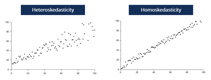
4/ ⚖️ Homoscedasticity: Fancy word, simple concept. We want the spread (or variance) of our residuals to be consistent across all levels of our independent variable(s). If not, we might have heteroscedasticity.
5/ 🔄 Linearity: The relationship between predictors and the outcome should be linear. If it's not, transformations of variables or non-linear models might be needed.
6/ 🤖 Leverage & Influence: Some data points can unduly influence our model. High-leverage points are outliers in the predictor space. Points with high influence affect the regression line substantially. Tools:
• Cook’s distance.
• Leverage plots.
7/ 🔥 Multicollinearity: When predictors are highly correlated, it's hard to tease apart their individual effects. This can make our model unstable. Tools:
• Variance Inflation Factor (VIF).
• Condition Index.
8/ 🔗 Autocorrelation: In time-series or spatial data, observations might not be independent, i.e., one observation could be correlated with a previous one. Durbin-Watson test helps detect this.
9/ 🛠️ Model Specification: Did we include all relevant predictors? Did we wrongly include unnecessary ones? Both can distort our findings.
10/ 🔄 Iterative Process: Diagnostics aren't a one-time check. As you adjust your model based on one diagnostic, recheck the others. It's all interconnected!
11/ 🎯 Conclusion: Diagnostics ensure our regression model's assumptions are met, enhancing reliability & accuracy. They help in troubleshooting & refining the model for the best fit. Like car maintenance, it's about prevention & timely intervention!
12/ 🌍 Engage: Fellow data enthusiasts, how do YOU approach diagnostics? Any favorite tools or methods? Share your insights!
(Note: While this thread offers a concise overview, regression diagnostics is a broad field. Those wanting to implement these methods should consult detailed statistical resources for in-depth understanding.)
#DataScience #RegressionAnalysis #Statistics

1/ 🚀 Introduction: Regression analysis is powerful, but like a car engine, it needs fine-tuning and regular checks. Diagnostics help us ensure our regression model runs smoothly and provides reliable results.
2/ 🔍 Residual Analysis: Residuals are the difference between the observed values and the values predicted by the model. Plotting residuals can reveal patterns indicating model inadequacies.
3/ 📊 Normality of Residuals: For many regression techniques, especially linear regression, residuals should be normally distributed. Tools:
• Histogram of residuals.
• Q-Q (Quantile-Quantile) plot.
4/ ⚖️ Homoscedasticity: Fancy word, simple concept. We want the spread (or variance) of our residuals to be consistent across all levels of our independent variable(s). If not, we might have heteroscedasticity.
5/ 🔄 Linearity: The relationship between predictors and the outcome should be linear. If it's not, transformations of variables or non-linear models might be needed.
6/ 🤖 Leverage & Influence: Some data points can unduly influence our model. High-leverage points are outliers in the predictor space. Points with high influence affect the regression line substantially. Tools:
• Cook’s distance.
• Leverage plots.
7/ 🔥 Multicollinearity: When predictors are highly correlated, it's hard to tease apart their individual effects. This can make our model unstable. Tools:
• Variance Inflation Factor (VIF).
• Condition Index.
8/ 🔗 Autocorrelation: In time-series or spatial data, observations might not be independent, i.e., one observation could be correlated with a previous one. Durbin-Watson test helps detect this.
9/ 🛠️ Model Specification: Did we include all relevant predictors? Did we wrongly include unnecessary ones? Both can distort our findings.
10/ 🔄 Iterative Process: Diagnostics aren't a one-time check. As you adjust your model based on one diagnostic, recheck the others. It's all interconnected!
11/ 🎯 Conclusion: Diagnostics ensure our regression model's assumptions are met, enhancing reliability & accuracy. They help in troubleshooting & refining the model for the best fit. Like car maintenance, it's about prevention & timely intervention!
12/ 🌍 Engage: Fellow data enthusiasts, how do YOU approach diagnostics? Any favorite tools or methods? Share your insights!
(Note: While this thread offers a concise overview, regression diagnostics is a broad field. Those wanting to implement these methods should consult detailed statistical resources for in-depth understanding.)
#DataScience #RegressionAnalysis #Statistics

• • •
Missing some Tweet in this thread? You can try to
force a refresh