Matrix factorizations are the pinnacle results of linear algebra.
From theory to applications, they are behind many theorems, algorithms, and methods. However, it is easy to get lost in the vast jungle of decompositions.
This is how to make sense of them.
From theory to applications, they are behind many theorems, algorithms, and methods. However, it is easy to get lost in the vast jungle of decompositions.
This is how to make sense of them.

We are going to study three matrix factorizations:
1. the LU decomposition,
2. the QR decomposition,
3. and the Singular Value Decomposition (SVD).
First, we'll take a look at LU.
1. the LU decomposition,
2. the QR decomposition,
3. and the Singular Value Decomposition (SVD).
First, we'll take a look at LU.
1. The LU decomposition.
Let's start at the very beginning: linear equation systems.
Linear equations are surprisingly effective in modeling real-life phenomena: economic processes, biochemical systems, etc.
Let's start at the very beginning: linear equation systems.
Linear equations are surprisingly effective in modeling real-life phenomena: economic processes, biochemical systems, etc.

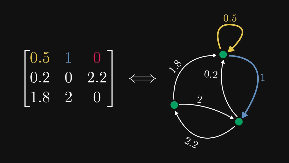
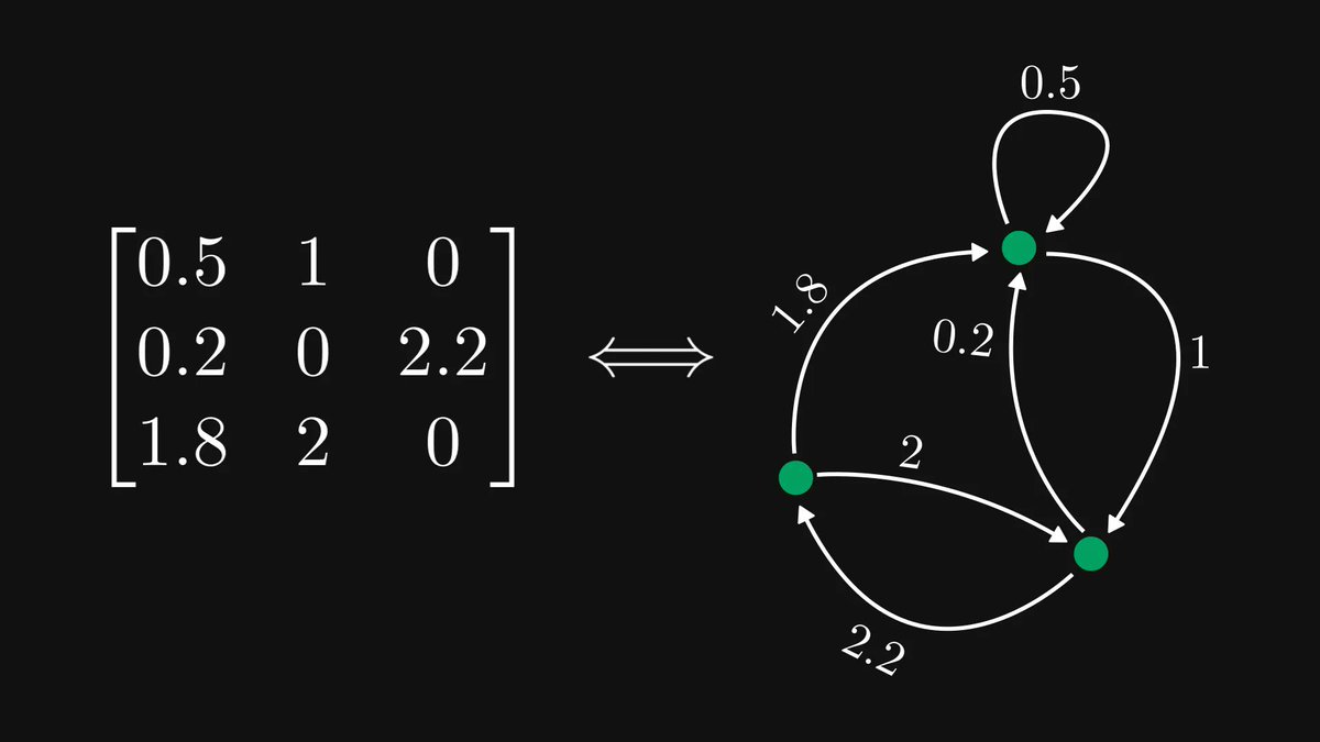
To simplify the notation, we can represent linear equations in a matrix form.
𝐴 holds the coefficients, 𝑥 holds the solution.
How can we solve this?
𝐴 holds the coefficients, 𝑥 holds the solution.
How can we solve this?

By multiplying the equations with scalars and subtracting them from each other, we can (usually) transform the system into an upper triangular form.
This is called Gaussian elimination.
The resulting system is easy to solve: solve the last equation, then move up progressively.
This is called Gaussian elimination.
The resulting system is easy to solve: solve the last equation, then move up progressively.

As it turns out, Gaussian elimination is equivalent to multiplying 𝐴 by a lower diagonal matrix.
This gives the famous LU decomposition, factoring 𝐴 into the product of a lower and an upper diagonal matrix.
This gives the famous LU decomposition, factoring 𝐴 into the product of a lower and an upper diagonal matrix.

Thus, LU is the same as solving a linear equation.
The LU decomposition can be performed whenever Gaussian elimination can, and it is vital in many applications, for instance, computing determinants or inverting matrices.
The LU decomposition can be performed whenever Gaussian elimination can, and it is vital in many applications, for instance, computing determinants or inverting matrices.
2. The QR decomposition.
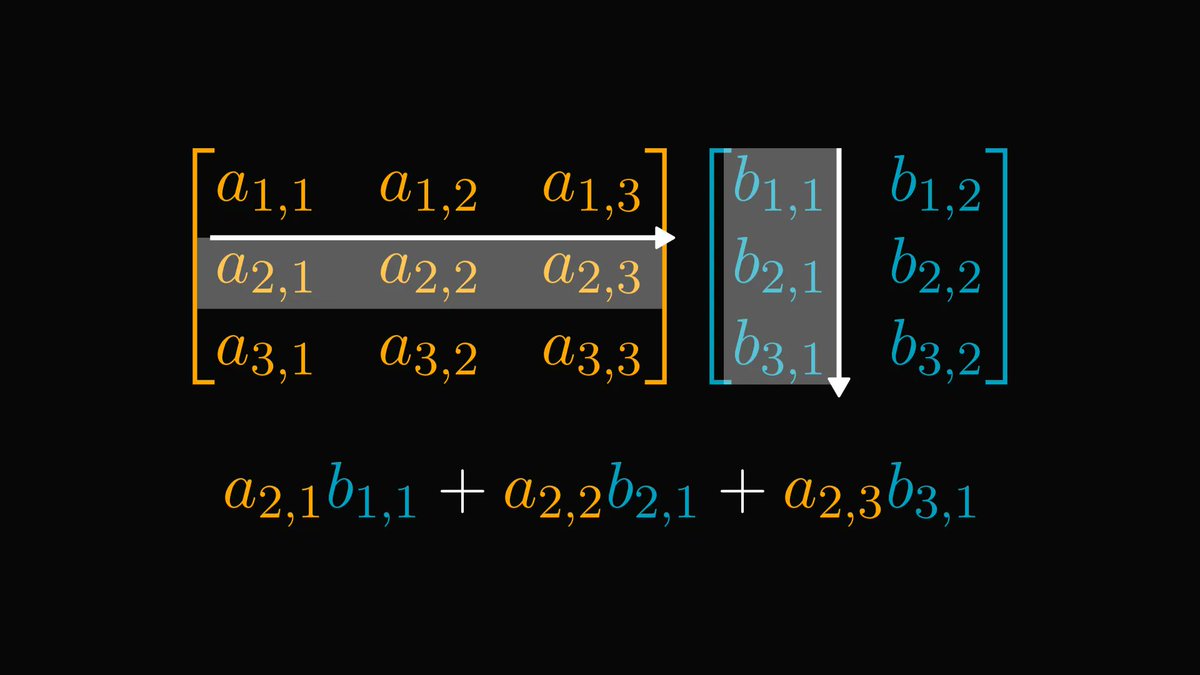
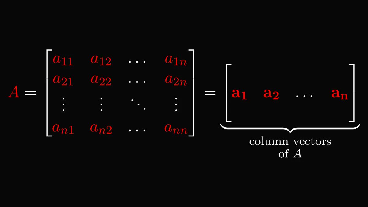
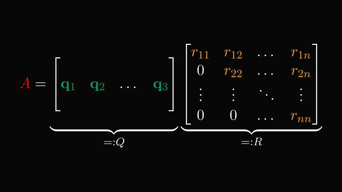
There are more than one ways to think about matrices. Previously, we viewed them as linear equations, but we can think about them as a horizontal stack of column vectors.
There are more than one ways to think about matrices. Previously, we viewed them as linear equations, but we can think about them as a horizontal stack of column vectors.
We can put these column vectors into the Gram-Schmidt orthogonalization process, yielding a set of orthonormal vectors that span the same space.

Just like Gaussian elimination, the Gram-Schmidt process can also be "vectorized", allowing us to use the resulting orthonormal system to factorize 𝐴 into the product of an orthogonal and an upper diagonal matrix.
Voila! This is the gist of QR decomposition.
Voila! This is the gist of QR decomposition.
Again, there are tons of applications, but the most significant one is the famous QR algorithm, using the QR decomposition to find the eigenvalues and the eigenvectors of arbitrary matrices.
en.wikipedia.org/wiki/QR_algori…
en.wikipedia.org/wiki/QR_algori…
3. The Singular Value Decomposition.
SVD is undoubtedly one of the pinnacle results of linear algebra, omnipresent in computer science and machine learning. For instance, the famous PCA algorithm is a version of SVD.
SVD is undoubtedly one of the pinnacle results of linear algebra, omnipresent in computer science and machine learning. For instance, the famous PCA algorithm is a version of SVD.
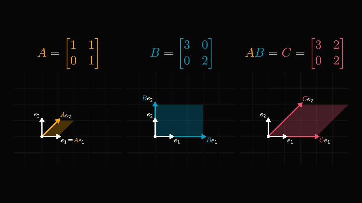
To understand the SVD, we should view matrices as linear transformations.
In essence, a linear transformation is a distortion of the underlying vector space, as illustrated below.
In essence, a linear transformation is a distortion of the underlying vector space, as illustrated below.

Although linear transformations can be complex, they are built from a few basic building blocks: rotations, reflections, stretchings.
A combination of rotations + reflections corresponds to a matrix whose columns are orthogonal.
Stretchings correspond to diagonal matrices.
A combination of rotations + reflections corresponds to a matrix whose columns are orthogonal.
Stretchings correspond to diagonal matrices.
On the level of transformations, SVD says that every transformation is a composition of
1. a rotations + reflections combo,
2. a stretching,
3. and a final rotations + reflections combo,
in that order.
1. a rotations + reflections combo,
2. a stretching,
3. and a final rotations + reflections combo,
in that order.

Translating it to the language of matrices, we obtain the factorization of 𝐴 into orthogonal and diagonal matrices.
This is an extremely strong result. Like the prime factorization theorem of integers, just for matrices.
(SVD works for non-square matrices as well.)
This is an extremely strong result. Like the prime factorization theorem of integers, just for matrices.
(SVD works for non-square matrices as well.)

SVD is everywhere in linear algebra. For instance, we can
1. generalize the notion of the inverse matrix to non-square matrices,
2. reduce the dimensionality of data,
3. approximate matrices with low-rank ones,
and many more.
1. generalize the notion of the inverse matrix to non-square matrices,
2. reduce the dimensionality of data,
3. approximate matrices with low-rank ones,
and many more.
This is just the tip of the iceberg. If you are in more about the beauties of linear algebra, check out my Mathematics of Machine Learning book!
Understanding mathematics will make you a better engineer, and I want to help you with that.
amazon.com/Mathematics-Ma…
Understanding mathematics will make you a better engineer, and I want to help you with that.
amazon.com/Mathematics-Ma…
• • •
Missing some Tweet in this thread? You can try to
force a refresh