Thread by @TivadarDanka

The single biggest argument about statistics: is probability frequentist or Bayesian?

It's neither, and I'll explain why.

Buckle up. Deep-dive explanation incoming.

First, let's look at what is probability.

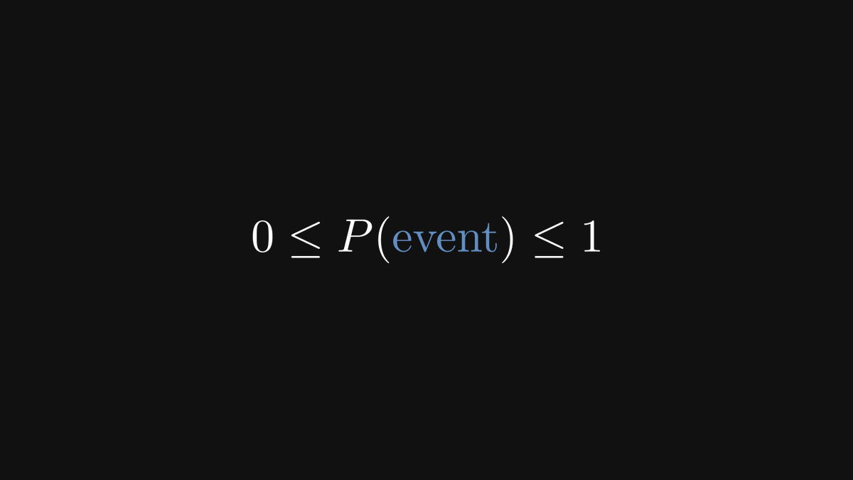
Probability quantitatively measures the likelihood of events, like rolling six with a dice. It's a number between zero and one. This is independent of interpretation; it’s a rule set in stone.

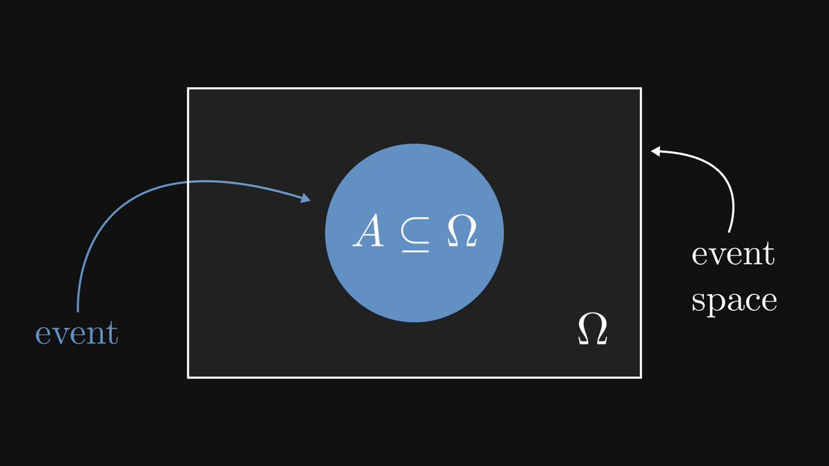
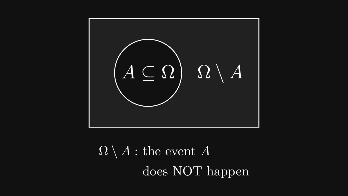
In the language of probability theory, the events are formalized by sets within an event space.

The event space is also a set, usually denoted by Ω.)

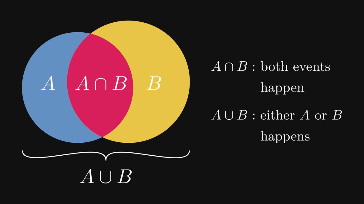
The union and intersection of sets can be translated into the language of events.

The intersection of two events expresses an outcome where both events happen simultaneously. (For instance, a dice roll can be both less than 4 and an odd number.)

We can also take the complement of an event, expressing when it does NOT happen.

So, probability is a function that takes a set and returns a number between 0 and 1.

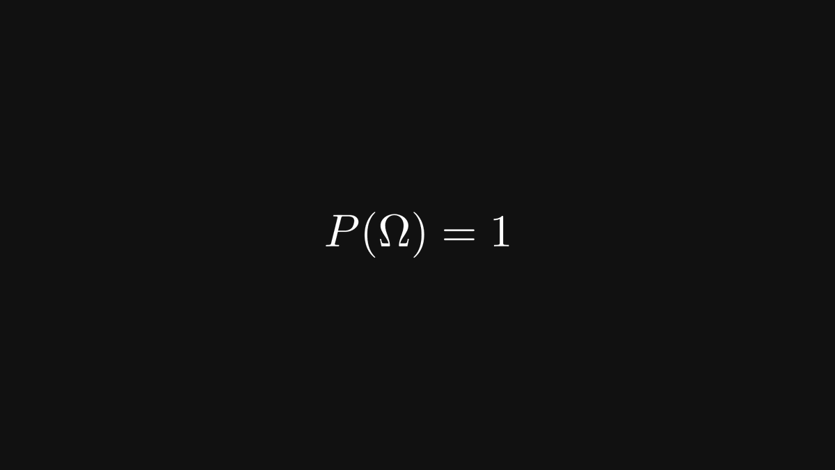
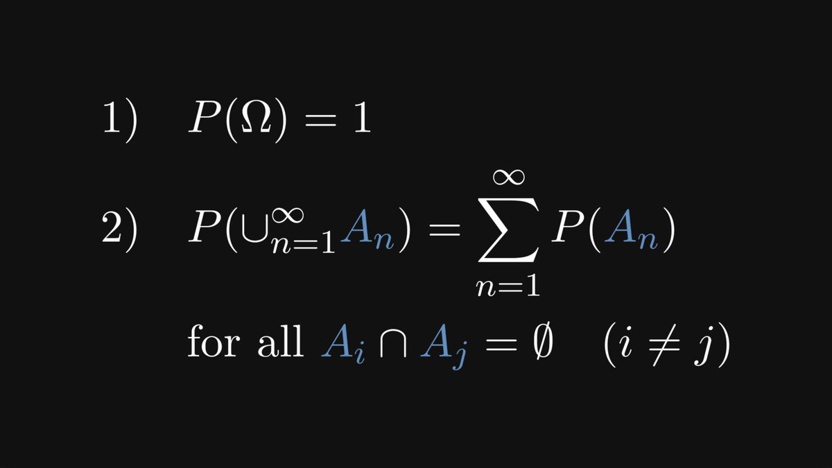
There are two fundamental properties we expect from probability. First, the probability of the entire event space must be 1.

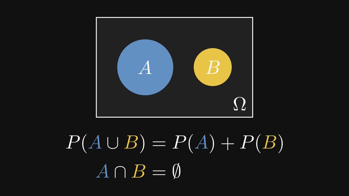
Second, that the probability of mutually exclusive events is the sum of their probabilities.

Intuitively, this is clear.

In fact, this is true for any countable collection of mutually exclusive events.

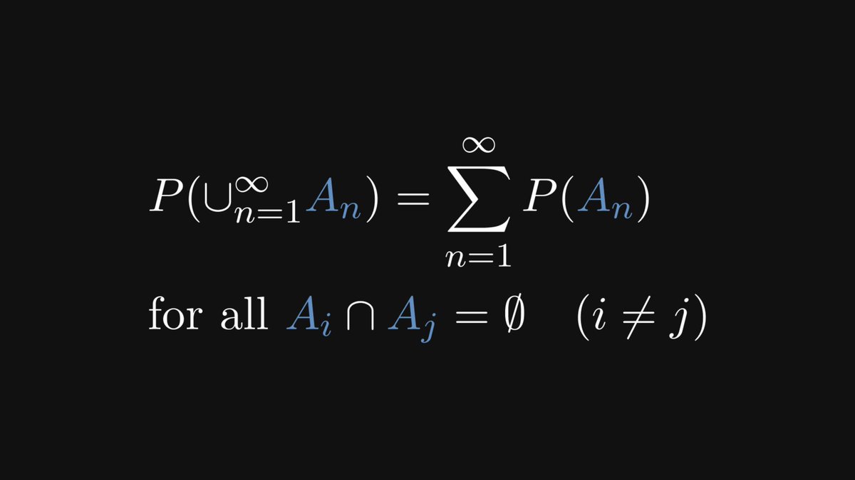
These two properties can be used to define probability!

Mathematically speaking, any measure that satisfies these two axioms is a probability measure.

These are called Kolmogorov’s axioms. Every result in probability theory and statistics is a consequence of them.

Let's see some probabilistic models!

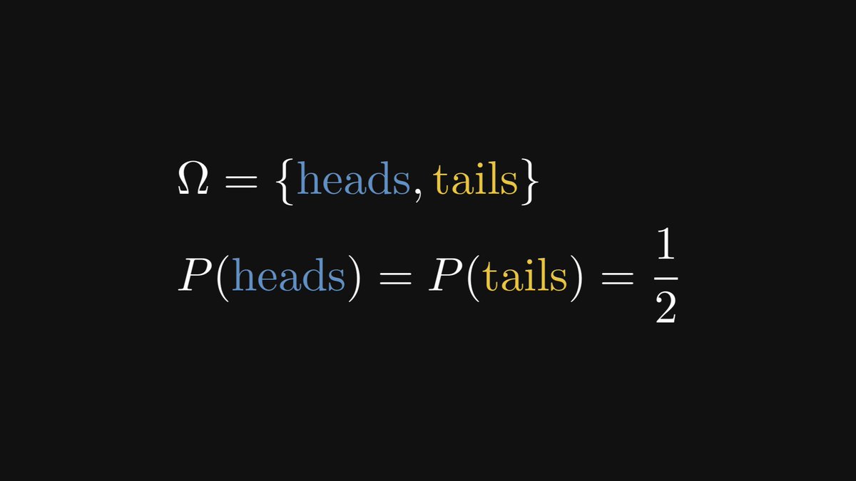
1. Tossing a fair coin. This is the simplest possible example. There are two possible outcomes, both having the same probability.

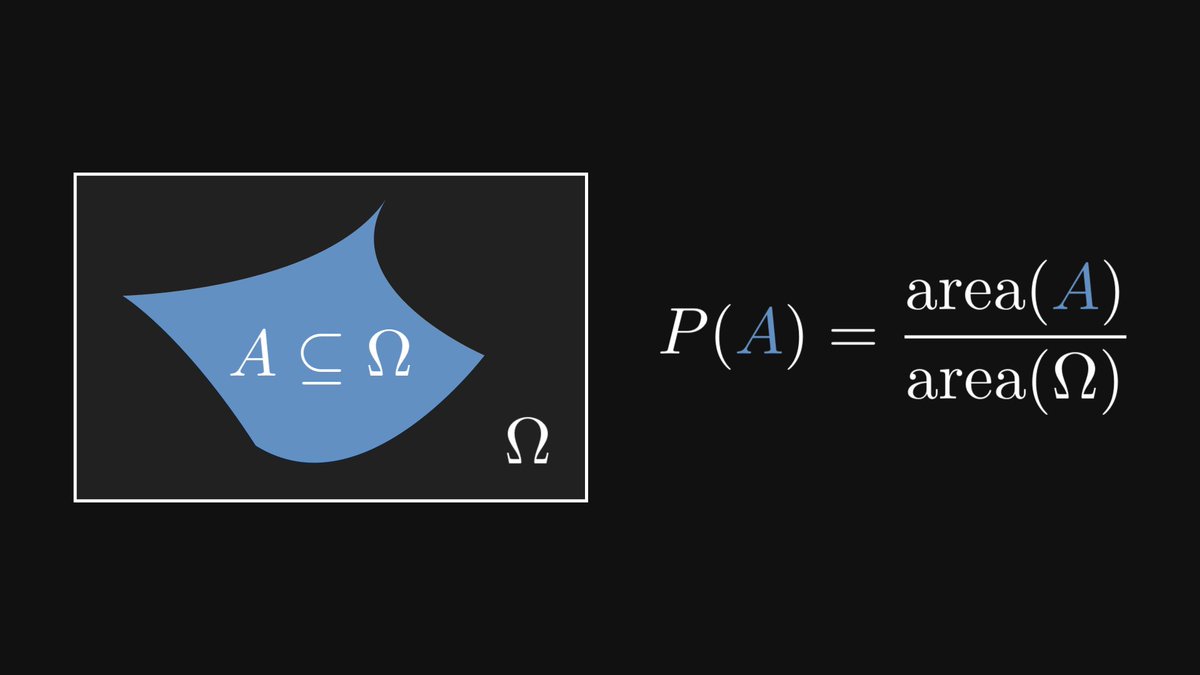
2. Throwing darts. Suppose that we are throwing darts at a large wall in front of us, which is our event space. (We'll always hit the wall.)

If we throw the dart randomly, the probability of hitting a certain shape is proportional to the shape's area.

Note that at this point, there is no frequentist or a Bayesian interpretation yet!

Probability is a well-defined mathematical object. This concept is separated from how probabilities are assigned.

Now comes the part that has been fueling debates for decades.

How can we assign probabilities? There are (at least) two schools of thought, constantly in conflict with each other.

Let's start with the frequentist school.

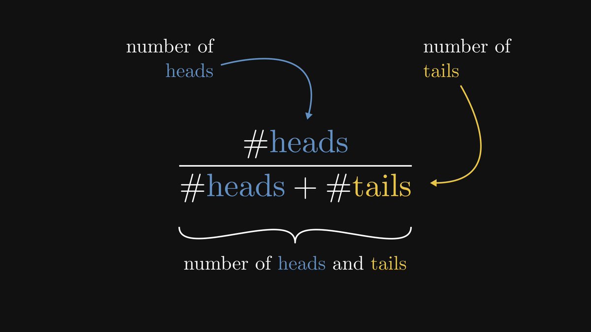
Suppose that we repeatedly perform a single experiment, counting the number of occurrences of the possible events. Say, we are tossing a coin and count the number of times it turns up heads.

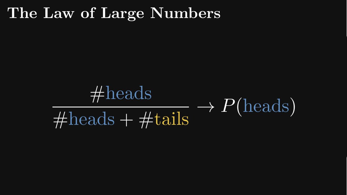
The ratio of the heads and the tosses is called “the relative frequency of heads”.

As the number of observations grows, the relative frequency will converge to the true probability.

This is not an interpretation of probability. This is a mathematically provable fact, independent of interpretations. (A special case of the famous Law of Large Numbers.)

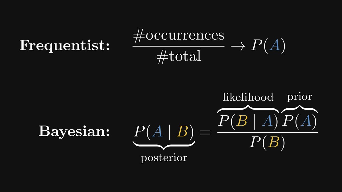
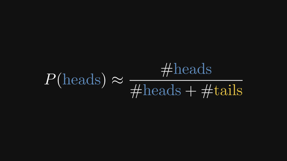
Frequentists leverage this to build probabilistic models. For example, if we toss a coin n times and heads come up exactly k times, then the probability of heads is estimated to be k/n.

On the other hand, the Bayesian school argues that such estimations are wrong, because probabilities are not absolute, but a measure of our current beliefs.

This is way too abstract, so let's elaborate.

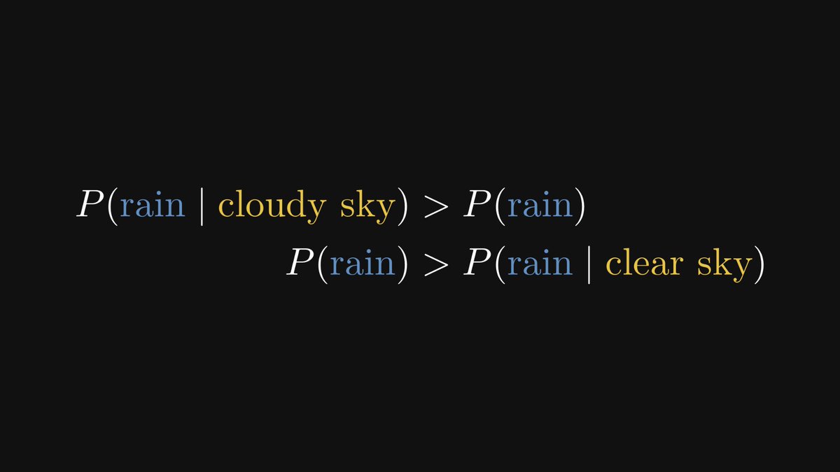
In probabilistic models, observing certain events can influence our beliefs about others. For instance, if the sky is clear, the probability of rain goes down. If it’s cloudy, the same probability goes up.

This is expressed in terms of conditional probabilities.

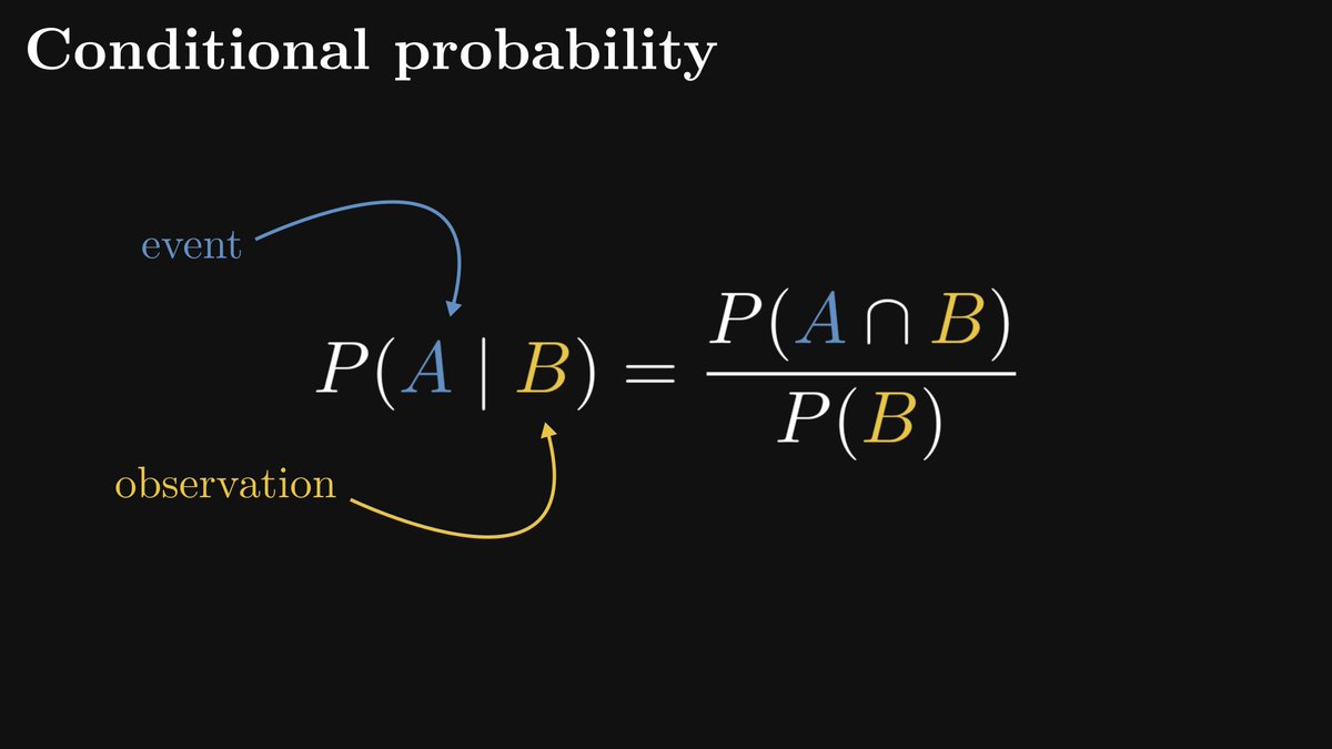
With conditional probabilities, we can quantify our intuition about the relation of rain and the clouds in the sky.

Conditional probabilities allow us to update our probabilistic model in light of new information. This is called the Bayes formula, hence the terminology "Bayesian statistics".

Again, this is a mathematically provable fact, not an interpretation.

Let's stick to our coin-tossing example to show how this works in practice. Regardless of the actual probabilities, 90 heads from 100 tosses is a possible outcome in (almost) every case.

Is the coin biased, or were we just lucky? How can we tell?

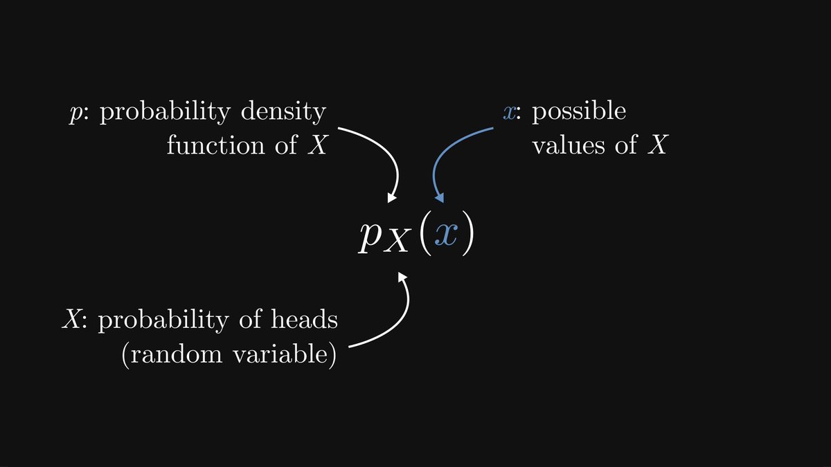
In Bayesian statistics, we treat our probability-to-be-estimated as a random variable. Thus, we are working with probability distributions or densities.

Yes, I know. The probability of probability. It’s kind of an Inception-moment, but you’ll get used to it.

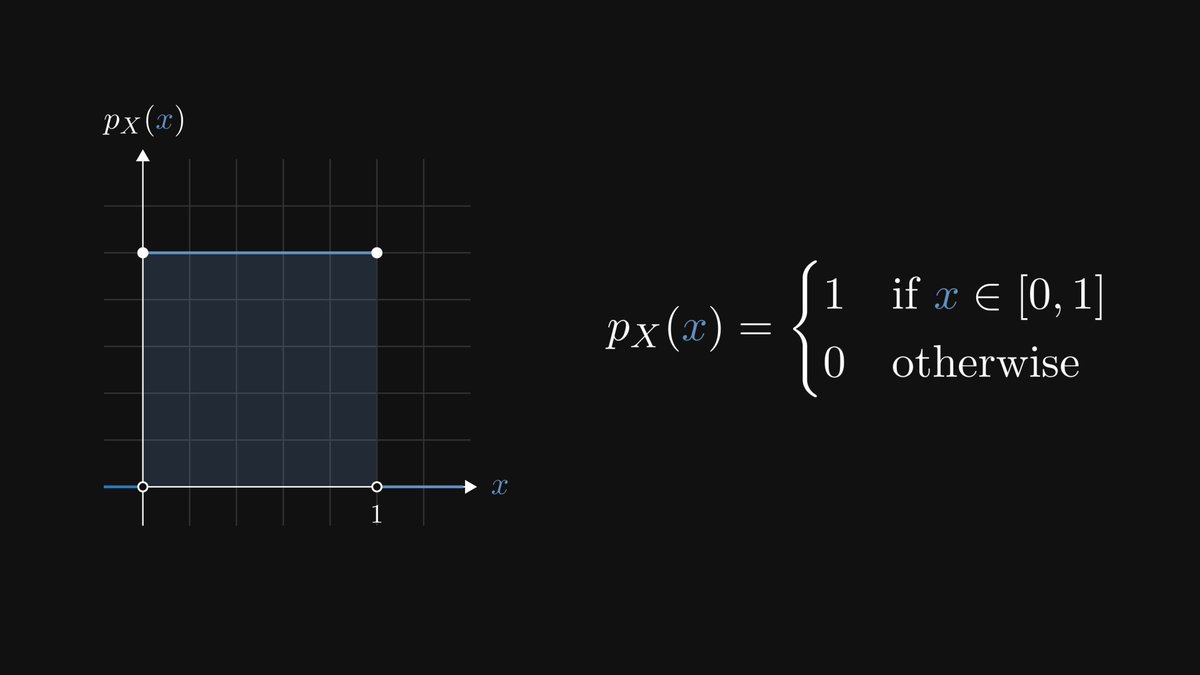
Our prior assumption about the probability is called, well, the prior.

For instance, if we know absolutely nothing about our coin, we assume this to be uniform.

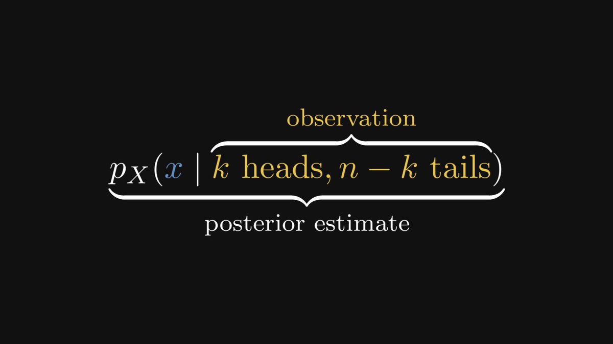
What we want is to include the experimental observations in our estimation, which is expressed in terms of conditional probabilities.

This is called posterior estimation.

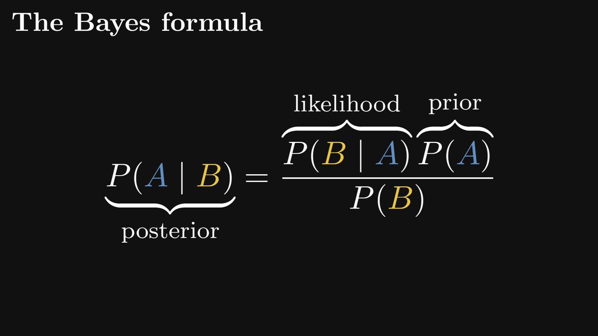
The Bayes formula connects the prior and the likelihood to the posterior.

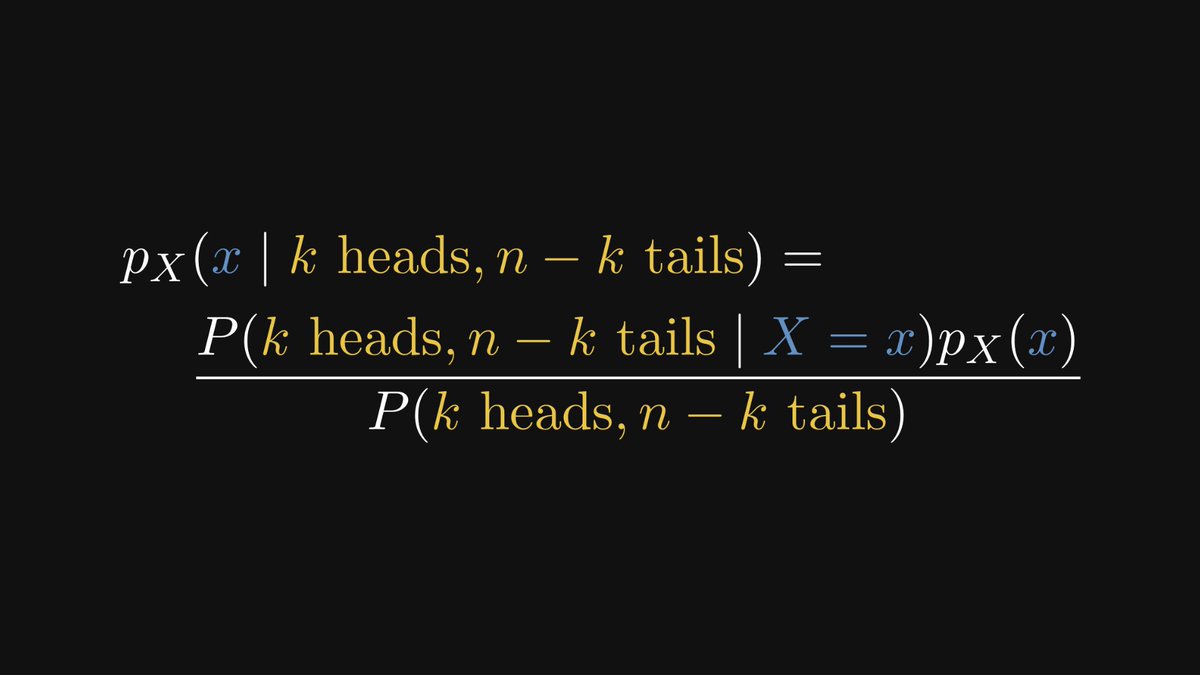
Don't worry if this seems complex! We'll unravel it term by term.

There are three terms on the right side: the likelihood, the prior, and the evidence.

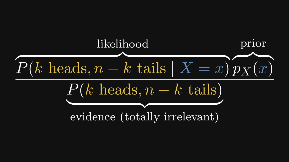
In pure English,

• the likelihood describes the probability of the observation given the model parameter,
• the prior describes our assumptions about the parameter before the observation,
• and the evidence is the total probability of our observation.

Bad news: the evidence can be impossible to evaluate. Good news: we don’t have to! We find the parameter estimate by maximizing the posterior, and as the evidence doesn’t depend on the parameter at all, we can simply omit it.

Back to our coin-tossing example. Given the probability of heads, the likelihood can be computed using simple combinatorics.

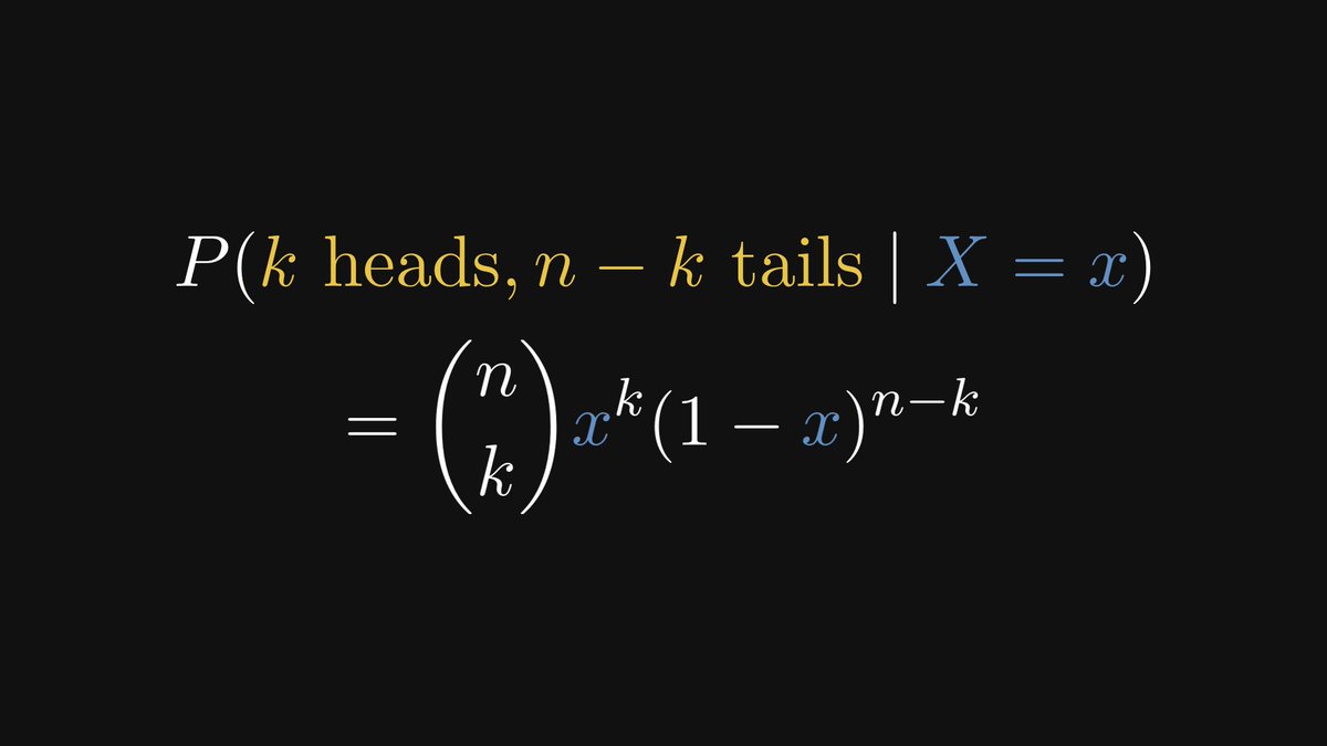
After this, we get a concrete formula for the posterior density.

(The symbol ∝ reads as “proportional to”, and we write this instead of equality because of the omitted denominator.)

To sum up: as a mathematical concept, probability is independent of interpretation. The question of frequentist vs. Bayesian comes up when we are building probabilistic models from data.

Is the Bayesian viewpoint better than the frequentist one?

No. It's just different. In certain situations, frequentist estimations are perfectly enough. In others, Bayesian methods have the advantage. Use the right tool for the task, and don't worry about the rest.

If you liked this thread, you will love The Palindrome, my weekly newsletter on Mathematics and Machine Learning.

Join 19,000+ curious readers here: thepalindrome.org