A question we never ask:
"How large is that number in the Law of Large Numbers?"
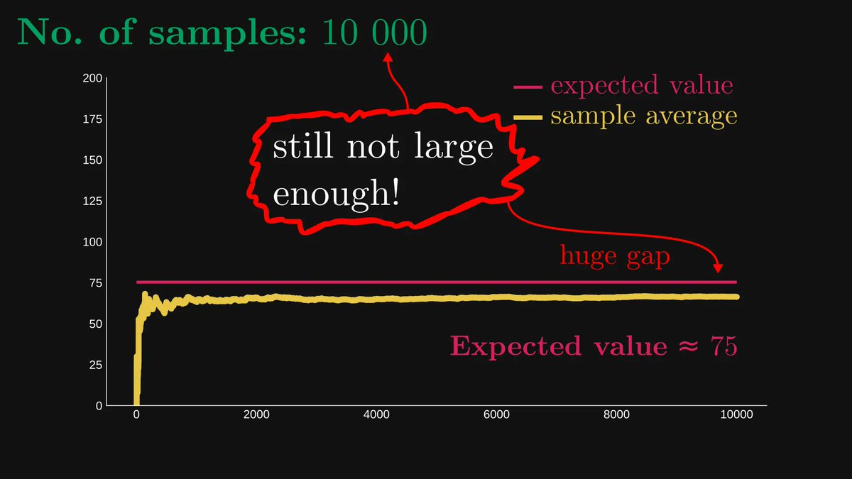
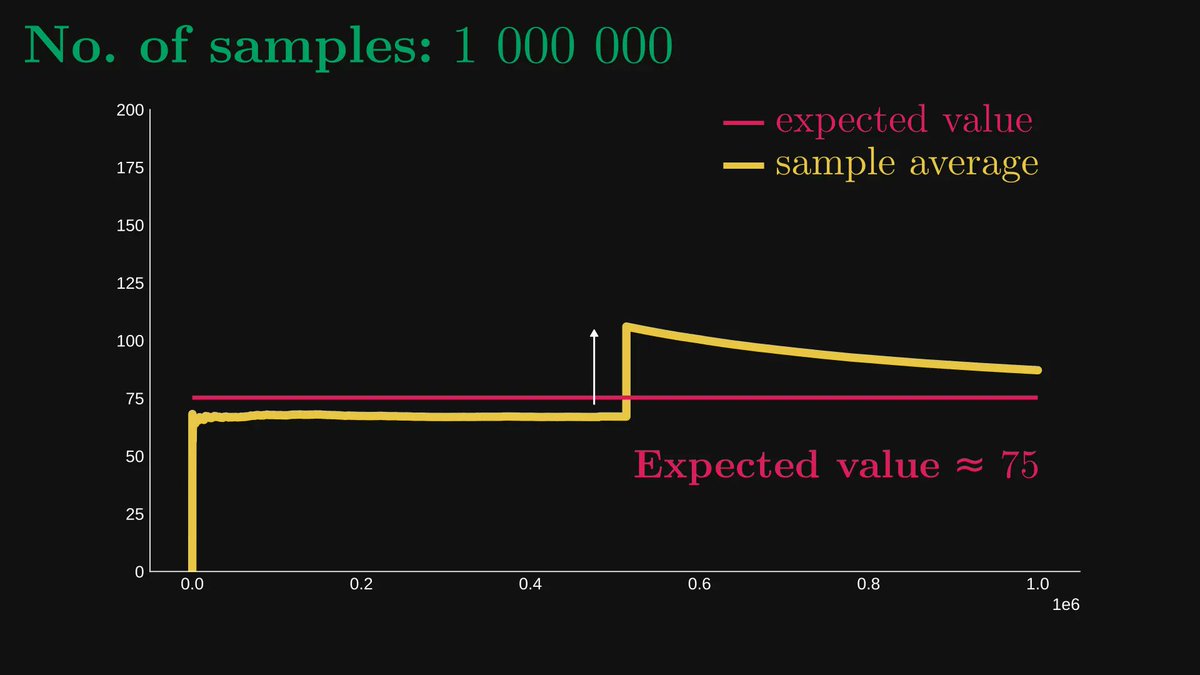
Sometimes, a thousand samples are large enough. Sometimes, even ten million samples fall short.
How do we know? I'll explain.
"How large is that number in the Law of Large Numbers?"
Sometimes, a thousand samples are large enough. Sometimes, even ten million samples fall short.
How do we know? I'll explain.
First things first: the law of large numbers (LLN).
Roughly speaking, it states that the averages of independent, identically distributed samples converge to the expected value, given that the number of samples grows to infinity.
We are going to dig deeper.
Roughly speaking, it states that the averages of independent, identically distributed samples converge to the expected value, given that the number of samples grows to infinity.
We are going to dig deeper.
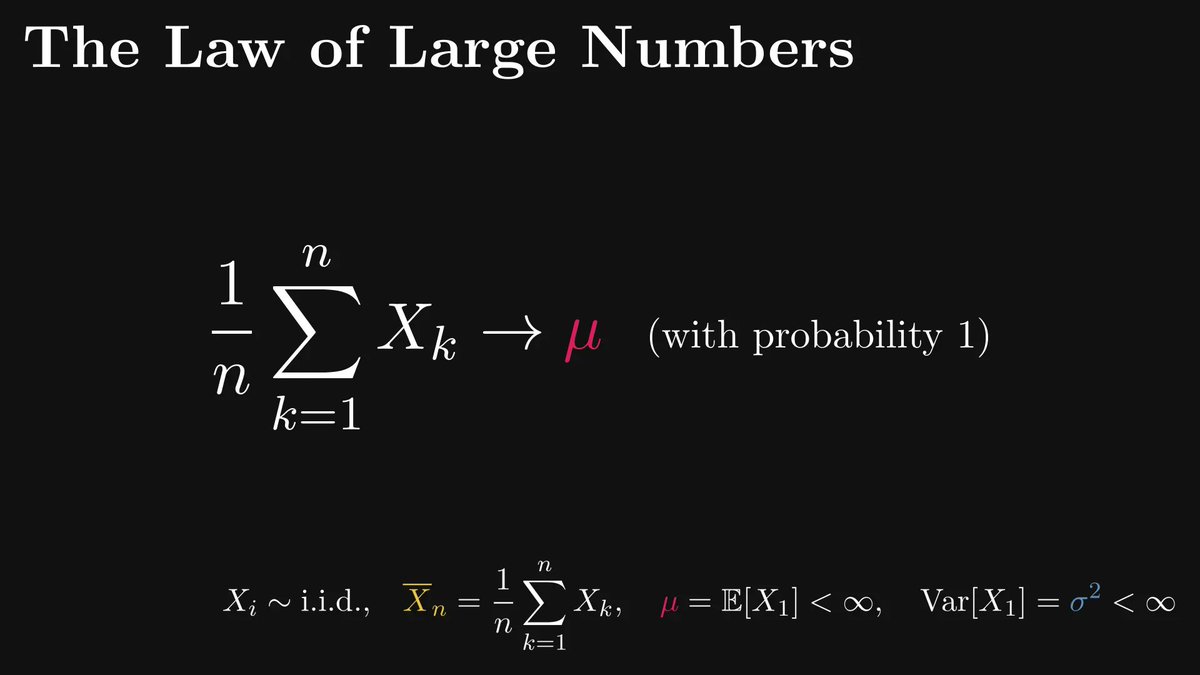
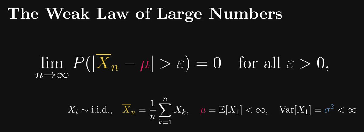
There are two kinds of LLN-s: weak and strong.
The weak law makes a probabilistic statement about the sample averages: it implies that the probability of "the sample average falling farther from the expected value than ε" goes to zero for any ε.
Let's unpack this.
The weak law makes a probabilistic statement about the sample averages: it implies that the probability of "the sample average falling farther from the expected value than ε" goes to zero for any ε.
Let's unpack this.
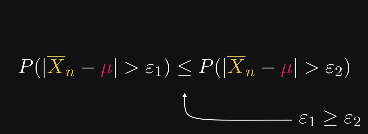
The quantity P(|X̅ₙ - μ| > ε) might be hard to grasp for the first time; but it just measures the distance of the sample mean from the true mean (that is, the expected value) in a probabilistic sense.
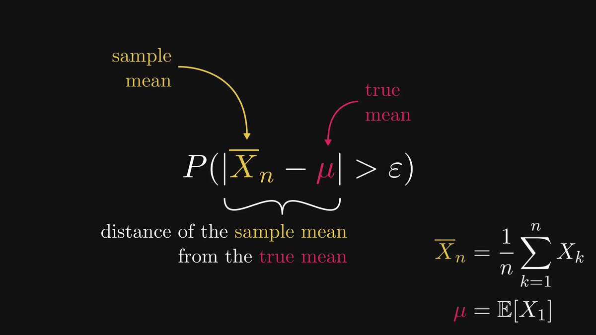
The smaller ε is, the larger the probabilistic distance.
Loosely speaking, the weak LLN means that the sample average equals the true average plus a distribution that gets more and more concentrated to zero.
In other terms, we have an asymptotic expansion!
Well, sort of. In the distributional sense, at least.
In other terms, we have an asymptotic expansion!
Well, sort of. In the distributional sense, at least.
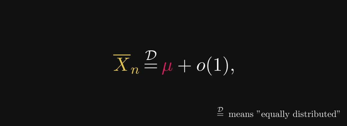
(You might be familiar with the small and big O notation; it’s the same but with probability distributions.
The term o(1) indicates a distribution that gets more and more concentrated to zero as n grows.
This is not precise, but we'll let that slide for the sake of simplicity.)
The term o(1) indicates a distribution that gets more and more concentrated to zero as n grows.
This is not precise, but we'll let that slide for the sake of simplicity.)
Does this asymptotic expansion tell us why we sometimes need tens of millions of samples, when a thousand seems to be enough on other occasions?
No. We have to go deeper.
Meet the Central Limit Theorem.
No. We have to go deeper.
Meet the Central Limit Theorem.
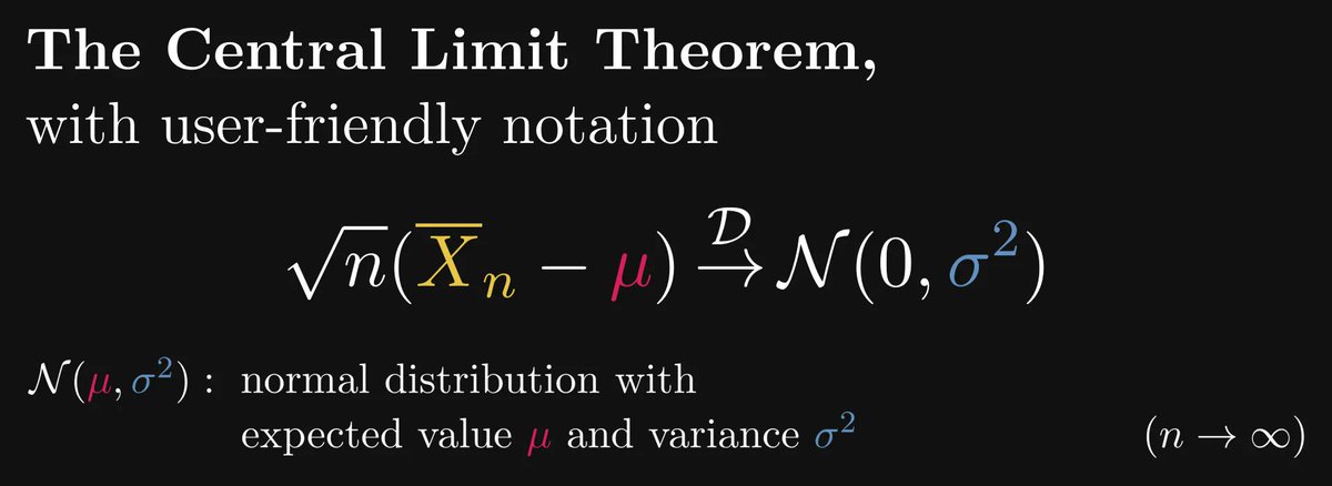
The central limit theorem (CLT) states that in a distributional sense, the √n-scaled centered sample averages converge to the standard normal distribution.
(The notion “centered” means that we subtract the expected value.)
(The notion “centered” means that we subtract the expected value.)
Let’s unpack it: in terms of an asymptotic expansion, the Law of Large Numbers and the Central Limit Theorem imply that the sample average equals the sum of
1) the expected value μ,
2) a scaled normal distribution,
3) and a distribution that vanishes faster than 1/√n.
1) the expected value μ,
2) a scaled normal distribution,
3) and a distribution that vanishes faster than 1/√n.
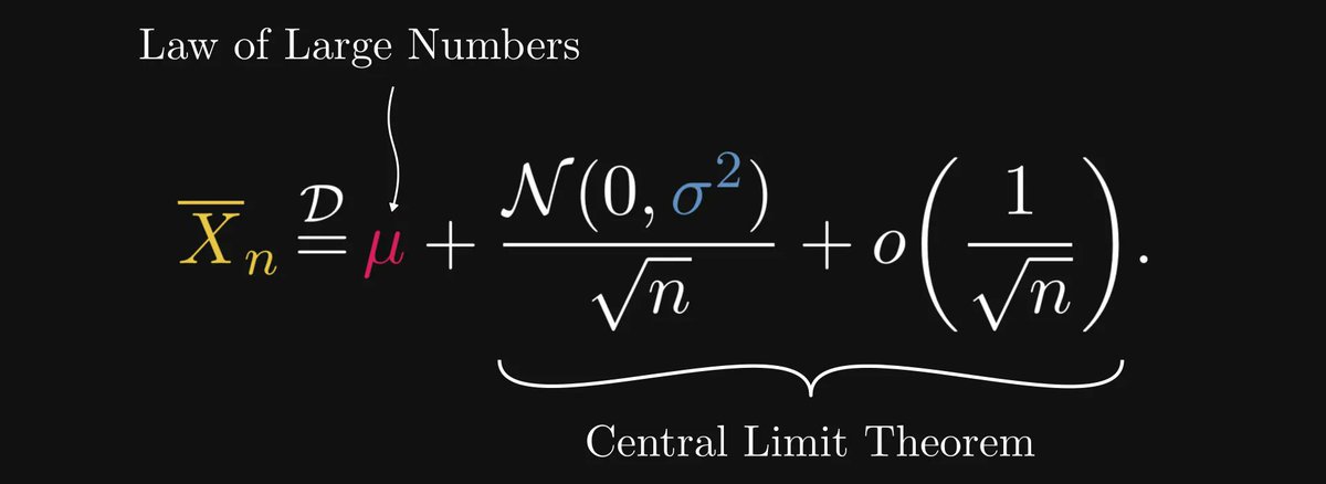
This expansion can be written in a simpler form by amalgamating the constants into the normal distribution.
More precisely, this is how the normal distribution behaves with respect to scaling:
More precisely, this is how the normal distribution behaves with respect to scaling:
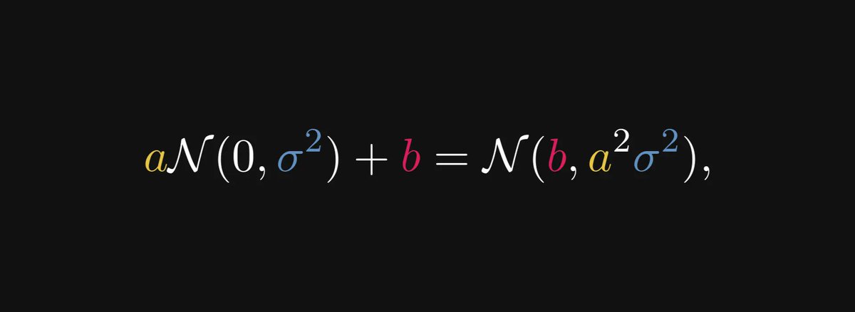
Thus, our asymptotic expansion takes the following form.
In other words, for large n, the sample average approximately equals a normal distribution with variance σ²/n.
In other words, for large n, the sample average approximately equals a normal distribution with variance σ²/n.
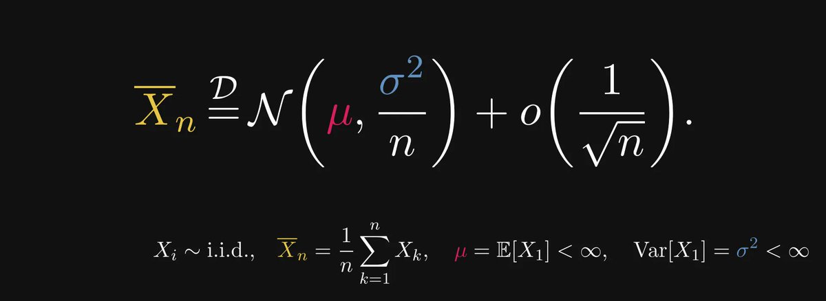
The larger the n, the smaller the variance; the smaller the variance, the more the normal distribution is concentrated around the expected value μ.
This is why sometimes one million samples are not enough.
Larger variance ⇒ more samples.
This is why sometimes one million samples are not enough.
Larger variance ⇒ more samples.
This post has been a collaboration with @levikul09, one of my favorite technical writers here.
Check out the full version:
thepalindrome.org/p/how-large-th…
Check out the full version:
thepalindrome.org/p/how-large-th…
If you liked this thread, you will love The Palindrome, my weekly newsletter on Mathematics and Machine Learning.
Join 19,000+ curious readers here: thepalindrome.org
Join 19,000+ curious readers here: thepalindrome.org
• • •
Missing some Tweet in this thread? You can try to
force a refresh