Thread by @_avichawla

A simple technique makes RAG ~32x memory efficient!

- Perplexity uses it in its search index
- Azure uses it in its search pipeline
- HubSpot uses it in its AI assistant

Let's understand how to use it in RAG systems (with code):

Today, let's build a RAG system that queries 36M+ vectors in <30ms using Binary Quantization.

Tech stack:
- @llama_index for orchestration
- @milvusio as the vector DB
- @beam_cloud for serverless deployment
- @Kimi_Moonshot Kimi-K2 as the LLM hosted on Groq

Let's build it!

Here's the workflow:

- Ingest documents and generate binary embeddings.
- Create a binary vector index and store embeddings in the vector DB.
- Retrieve top-k similar documents to the user's query.
- LLM generates a response based on additional context.

Let's implement this!

0️⃣ Setup Groq

Before we begin, store your Groq API key in a .env file and load it into your environment to leverage the world's fastest AI inference.

Check this 👇

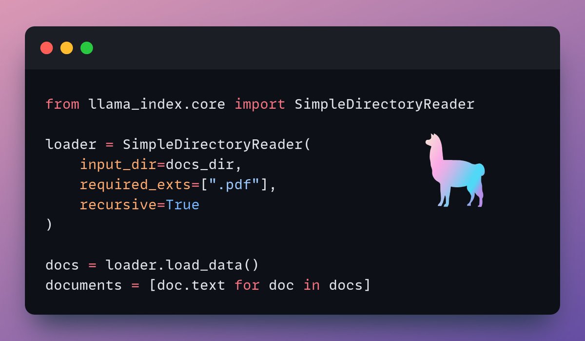
1️⃣ Load data

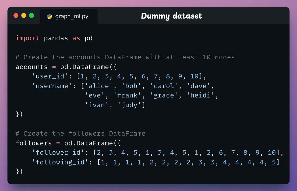
We ingest our documents using LlamaIndex's directory reader tool.

It can read various data formats including Markdown, PDFs, Word documents, PowerPoint decks, images, audio and video.

Check this 👇

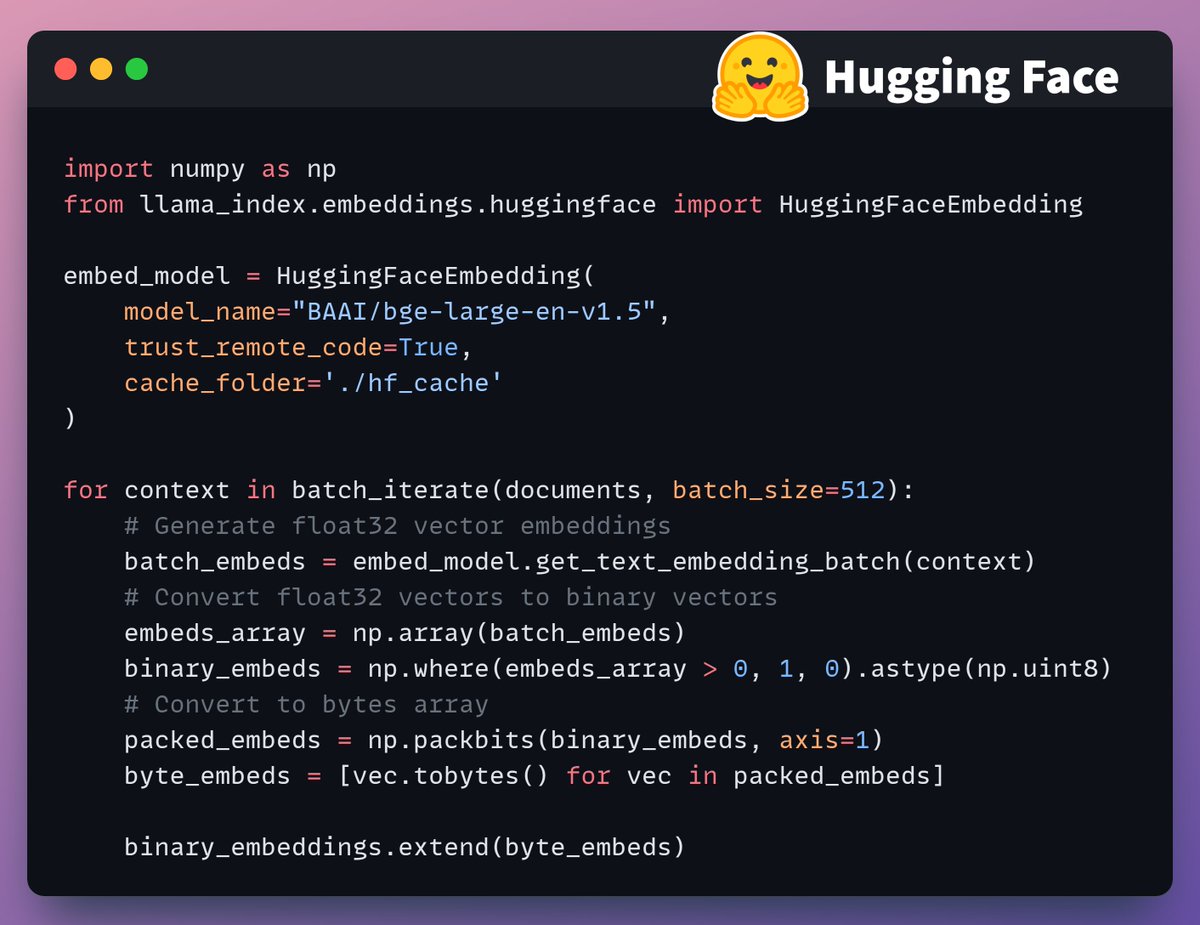
2️⃣ Generate Binary Embeddings

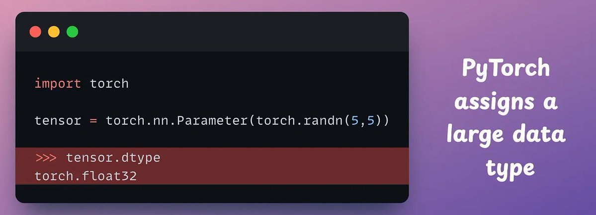
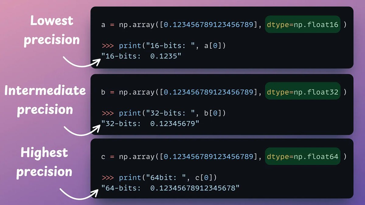
Next, we generate text embeddings (in float32) and convert them to binary vectors, resulting in a 32x reduction in memory and storage.

This is called binary quantization.

Check this implementation 👇

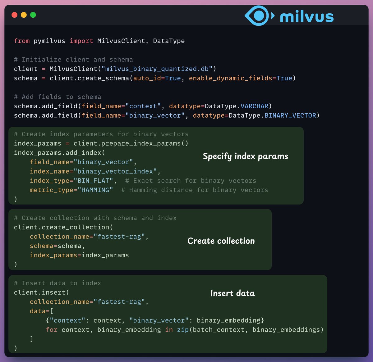
3️⃣ Vector indexing

After our binary quantization is done, we store and index the vectors in a Milvus vector database for efficient retrieval.

Indexes are specialized data structures that help optimize the performance of data retrieval operations.

Check this 👇

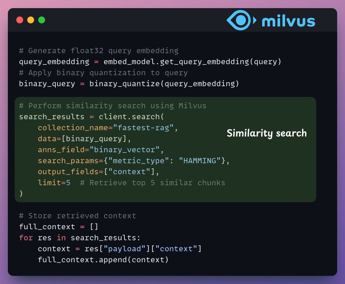
4️⃣ Retrieval

In the retrieval stage, we:

- Embed the user query and apply binary quantization to it.
- Use Hamming distance as the search metric to compare binary vectors.
- Retrieve the top 5 most similar chunks.
- Add the retrieved chunks to the context.

Check this👇

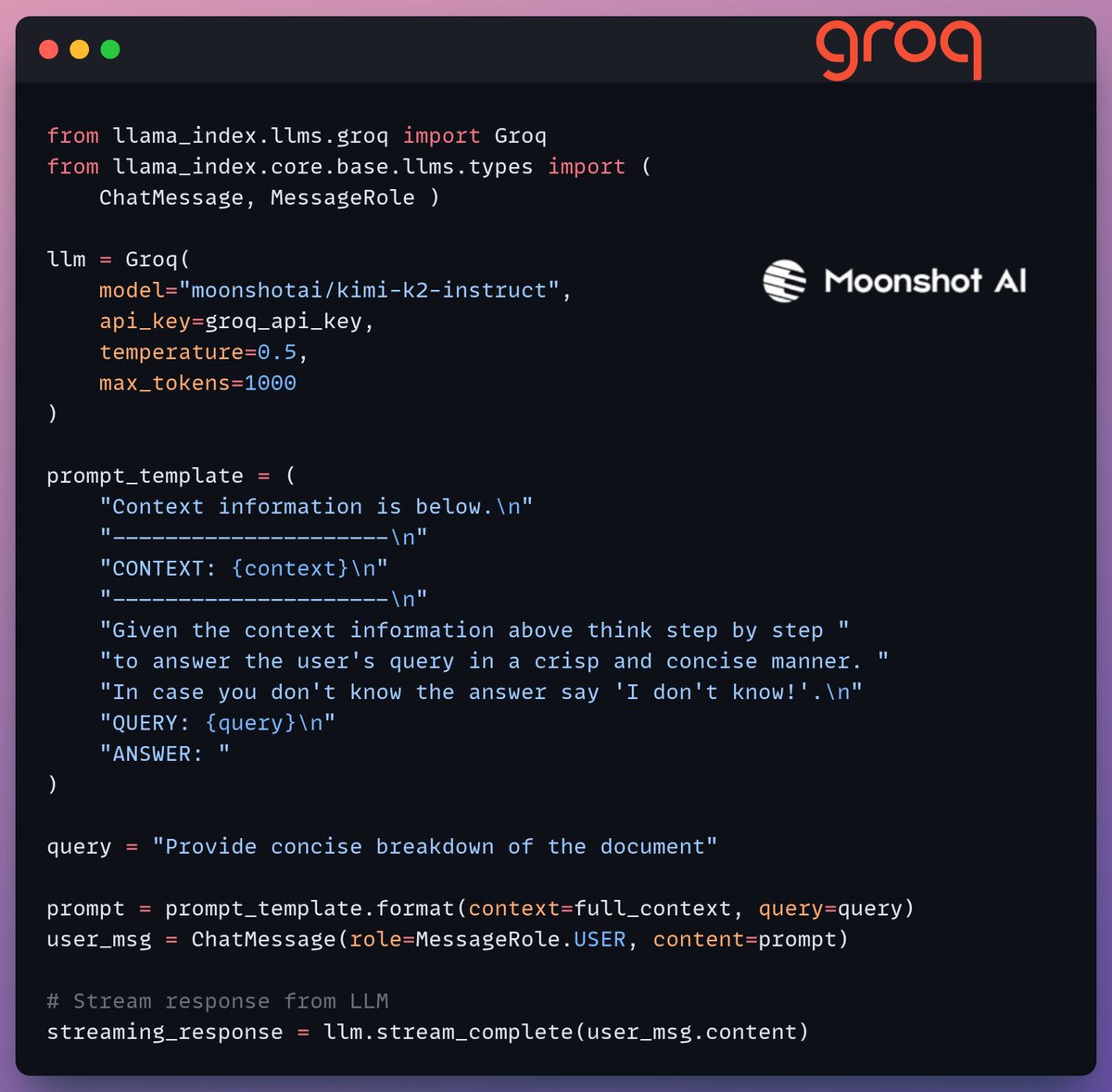
5️⃣ Generation

Finally, we build a generation pipeline using the Kimi-K2 instruct model, served on the fastest AI inference by Groq.

We specify both the query and the retrieved context in a prompt template and pass it to the LLM.

Check this 👇

6️⃣ Deployment with Beam

Beam enables ultra-fast serverless deployment of any AI workflow.

Thus, we wrap our app in a Streamlit interface, specify the Python libraries, and the compute specifications for the container.

Finally, we deploy the app in a few lines of code👇

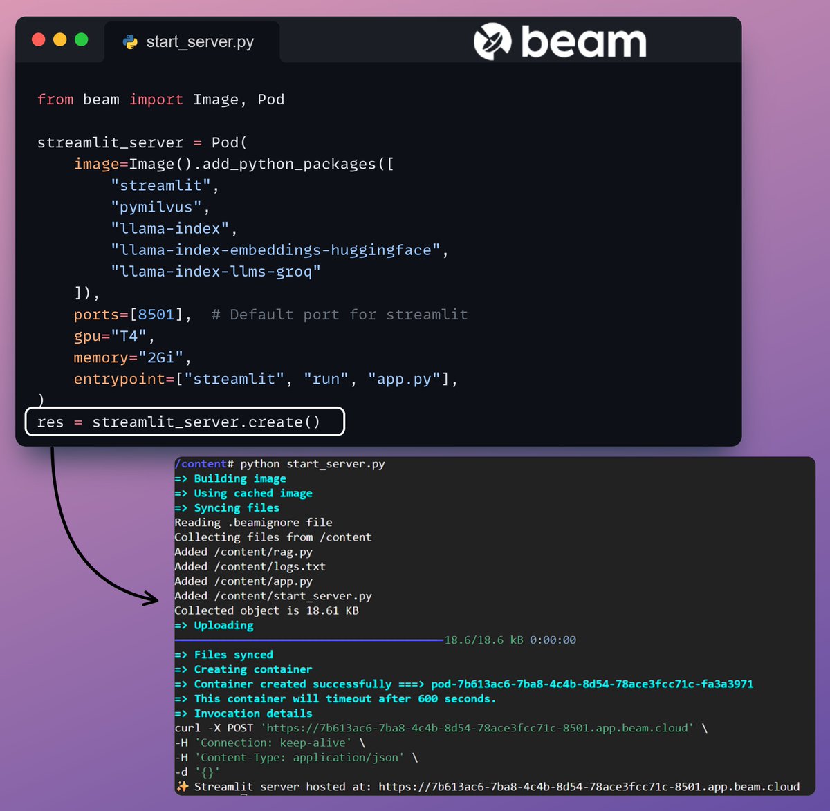
7️⃣ Run the app

Beam launches the container and deploys our streamlit app as an HTTPS server that can be easily accessed from a web browser.

Check this demo 👇

Moving on, to truly assess the scale and inference speed, we test the deployed setup over the PubMed dataset (36M+ vectors).

Our app:
- queried 36M+ vectors in <30ms.
- generated a response in <1s.

Check this demo👇

Done!

We just built the fastest RAG stack leveraging BQ for efficient retrieval and
using ultra-fast serverless deployment of our AI workflow.

Here's the workflow again for your reference 👇

That's a wrap!

If you found it insightful, reshare it with your network.

Find me → @_avichawla
Every day, I share tutorials and insights on DS, ML, LLMs, and RAGs.

https://twitter.com/1175166450832687104/status/1952256615215976745