BRILLIANT @GoogleDeepMind research.
Even the best embeddings cannot represent all possible query-document combinations, which means some answers are mathematically impossible to recover.
Reveals a sharp truth, embedding models can only capture so many pairings, and beyond that, recall collapses no matter the data or tuning.
🧠 Key takeaway
Embeddings have a hard ceiling, set by dimension, on how many top‑k document combinations they can represent exactly.
They prove this with sign‑rank bounds, then show it empirically and with a simple natural‑language dataset where even strong models stay under 20% recall@100.
When queries force many combinations, single‑vector retrievers hit that ceiling, so other architectures are needed.
4096‑dim embeddings already break near 250M docs for top‑2 combinations, even in the best case.
🛠️ Practical Implications
For applications like search, recommendation, or retrieval-augmented generation, this means scaling up models or datasets alone will not fix recall gaps.
At large index sizes, even very high-dimensional embeddings fail to capture all combinations of relevant results.
So embeddings cannot work as the sole retrieval backbone. We will need hybrid setups, combining dense vectors with sparse methods, multi-vector models, or rerankers to patch the blind spots.
This shifts how we should design retrieval pipelines, treating embeddings as one useful tool but not a universal solution.
🧵 Read on 👇
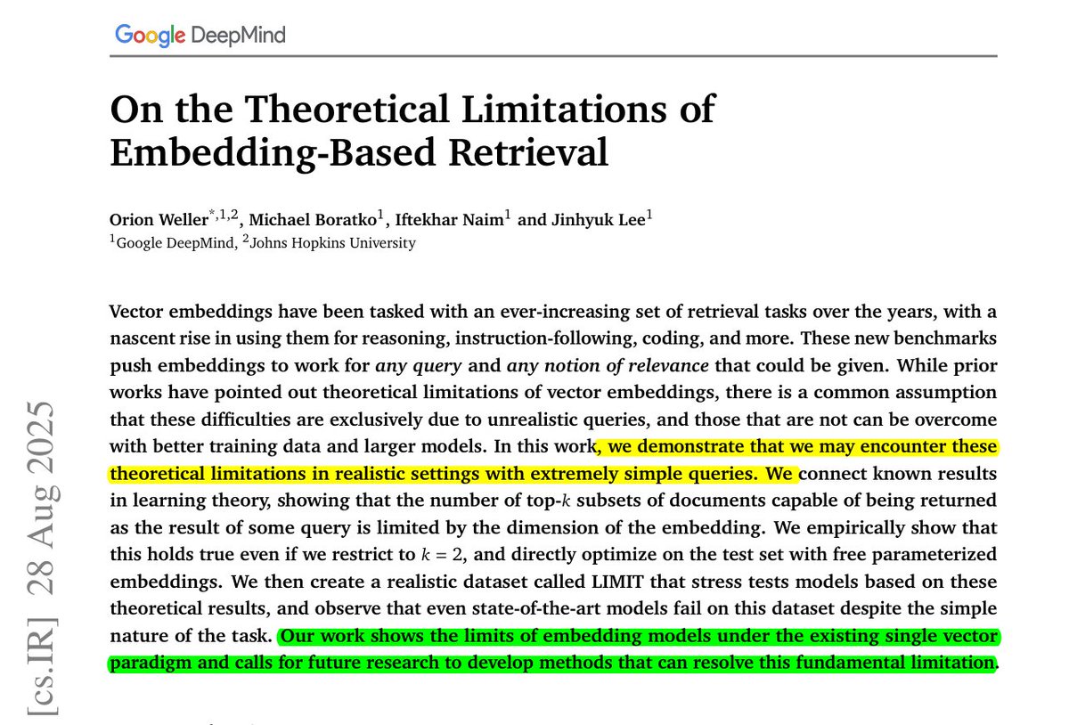
This figure explains LIMIT, a tiny natural-language dataset they built to test whether single-vector embeddings can represent all combinations of relevant documents for each query.
The left grid is the target relevance pattern, and the task is to rank exactly the k=2 correct documents for every query.
The right side shows the mapping into simple text, queries like “Who likes Quokkas?” paired with short bios such as “Jon Durben likes Quokkas and Apples,” so language complexity is not the challenge.
The key point, even with this simple setup, strong MTEB embedders stay under 20% recall@100, revealing a capacity limit of single-vector retrieval.
2. ⚙️ The core concepts
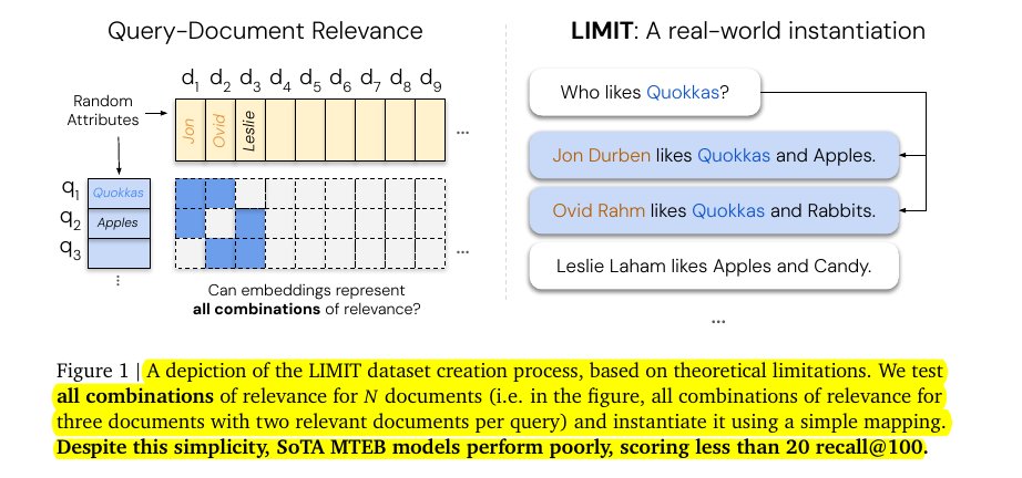
They formalize retrieval as a binary relevance matrix over queries and documents, then ask for a low‑rank score matrix that, for each query, puts relevant documents ahead of the others.
They show that “row‑wise order preserving” and “row‑wise thresholdable” are the same requirement for binary labels, so both describe the exact capacity a single‑vector model needs.
They connect that capacity to sign rank, which is the smallest dimension that can reproduce the positive or negative pattern of a matrix, and they derive tight lower and upper bounds on the needed embedding dimension from it.
A direct consequence is stark, for any fixed dimension d, there exist top‑k combinations no query embedding can ever retrieve, regardless of training data.
3. 🧪 Best‑case test, no language in the loop
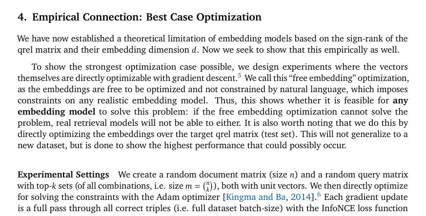
They remove language completely and directly optimize the document and query vectors against the target relevance matrix with full‑batch contrastive training, which is the friendliest possible setup for embeddings.
For k=2, they increase the number of documents until optimization cannot reach 100% accuracy, calling that cutoff the critical‑n for a given dimension.
The curve of critical‑n versus dimension fits a 3rd‑degree polynomial with r^2=0.999, which lets them extrapolate how scale pushes the ceiling.
The extrapolated breakpoints are 500K @ 512, 1.7M @ 768, 4M @ 1024, 107M @ 3072, 250M @ 4096, and this is already the best case any retriever could hope for.
4. 🧩 What LIMIT actually is
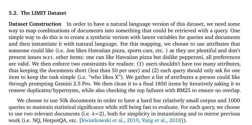
They build a natural‑language dataset that encodes all 2‑document combinations across a small pool, phrased as simple queries like “who likes X” and short biography‑style documents.
Each document lists fewer than 50 liked attributes to keep texts short, and each query asks for exactly 1 attribute, which keeps the language trivial and isolates the combination pressure.
They use 50K documents and 1000 queries, and pick 46 special documents because 46 choose 2 equals 1035, which is just above 1000, then they also provide a 46‑doc small split.
They randomize names and attributes, dedupe with lexical checks, and ensure every relevant pair appears somewhere, so the dataset is simple in wording but dense in combinations.
5. 📉 How current embedders fared
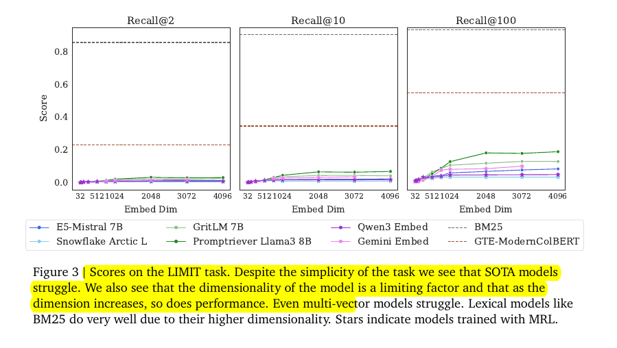
On the full LIMIT, leading single‑vector models struggle to even touch 20% recall@100, despite the plain language and the easy query form.
Performance grows with dimension but stays low, while a late‑interaction multi‑vector model does much better and a high‑dimensional sparse baseline, BM25, reaches about 93.6 recall@100 and GTE‑ModernColBERT sits near 54.8 recall@100.
This pattern matches the theory, more dimensions or more expressive matching buys more combinations, but a single compact vector hits limits fast.
6. 🪙 Even 46 docs are hard
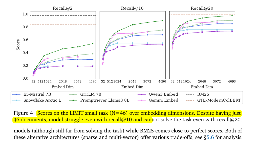
With just 46 documents, models still do not reach 100% even by recall@20, and recall@10 sits notably lower.
Concrete numbers help, Promptriever 4096 reaches 97.7 recall@20, GritLM 4096 reaches 90.5, and E5‑Mistral 4096 reaches 85.2, which is high but still not perfect for such a tiny pool.
With just 46 documents, models still do not reach 100% even by recall@20, and recall@10 sits notably lower.
Concrete numbers help, Promptriever 4096 reaches 97.7 recall@20, GritLM 4096 reaches 90.5, and E5‑Mistral 4096 reaches 85.2, which is high but still not perfect for such a tiny pool.
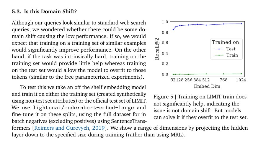
7. 🧪 Not a domain‑shift issue
Fine‑tuning an embedder on a matching training split barely moves the needle, with best gains only around 2.8 recall@10, so the failure is not because the language is unfamiliar.
Training on the test split lets the model overfit and reach near‑100% in this small case, which mirrors the free‑embedding result and confirms this is a capacity limit, not a distribution gap.
8. 🧮 Why the label pattern matters
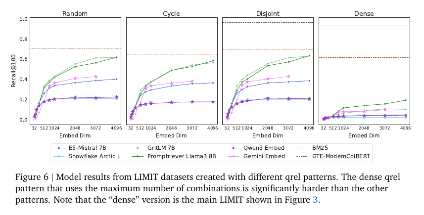
When the qrels are dense, meaning many document pairs co‑occur across queries, scores crash across models, which shows that combination count, not language tricks, drives the difficulty.
For example, E5‑Mistral drops from 40.4 recall@100 to 4.8, and GritLM loses about 50 absolute points moving to the dense pattern.
9. 🧱 What to use when single vectors hit the wall
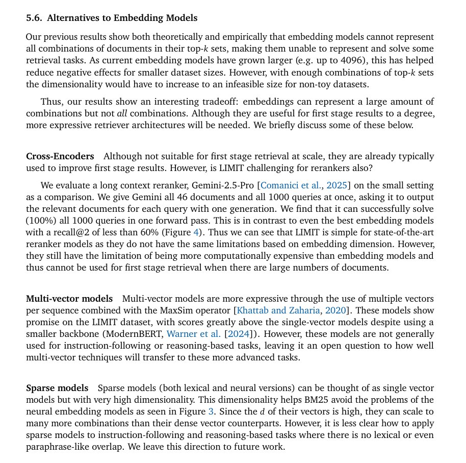
A long‑context reranker solved the small LIMIT with 100% accuracy by reading all 46 documents and 1000 queries together, which avoids the single‑vector bottleneck but costs more compute.
Multi‑vector late‑interaction retrieval lifts scores well above single‑vector baselines, and sparse term‑matching like BM25 stays strong because its effective dimension is huge compared to dense embeddings.
Paper –
Paper Title: "On the Theoretical Limitations of Embedding-Based Retrieval"arxiv.org/abs/2508.21038
Paper Title: "On the Theoretical Limitations of Embedding-Based Retrieval"arxiv.org/abs/2508.21038
• • •
Missing some Tweet in this thread? You can try to
force a refresh


