Post

How to get URL link on X (Twitter) App

On the Twitter thread, click on or icon on the bottom
Click again on or Share Via icon
Click on Copy Link to Tweet
Paste it above and click "Unroll Thread"!
More info at Twitter Help

Avi Chawla

@_avichawla

Sep 6, 2025 • 13 tweets • 4 min read • Read on X

Scrolly

Let's generate our own LLM fine-tuning dataset (100% local):

Before we begin, here's what we're doing today!

We'll cover:
- What is instruction fine-tuning?
- Why is it important for LLMs?

Finally, we'll create our own instruction fine-tuning dataset.

Let's dive in!

Once an LLM has been pre-trained, it simply continues the sentence as if it is one long text in a book or an article.

For instance, check this to understand how a pre-trained LLM behaves when prompted 👇

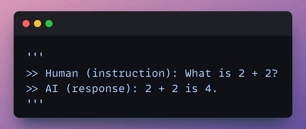
Generating a synthetic dataset using existing LLMs and utilizing it for fine-tuning can improve this.

The synthetic data will have fabricated examples of human-AI interactions.

Check this sample👇

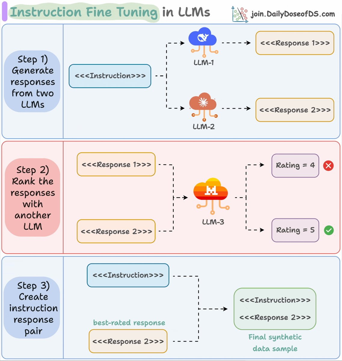
This process is called instruction fine-tuning.

Distilabel is an open-source framework that facilitates generating domain-specific synthetic text data using LLMs.

Check this to understand the underlying process👇

Next, let's look at the code.

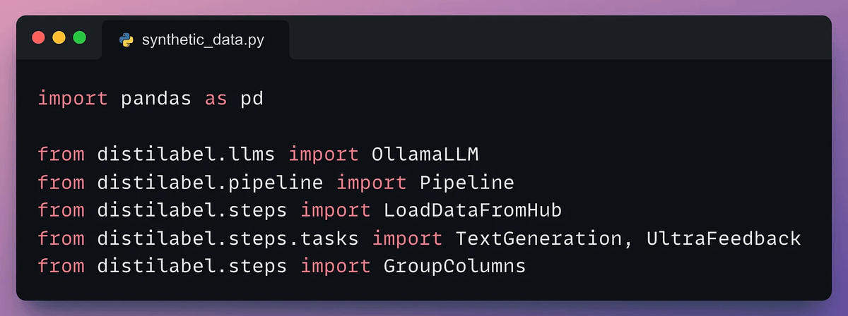
First, we start with some standard imports.

Check this👇

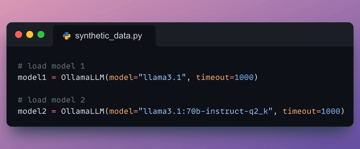
Moving on, we load the Llama-3 models locally with Ollama.

Here's how we do it👇

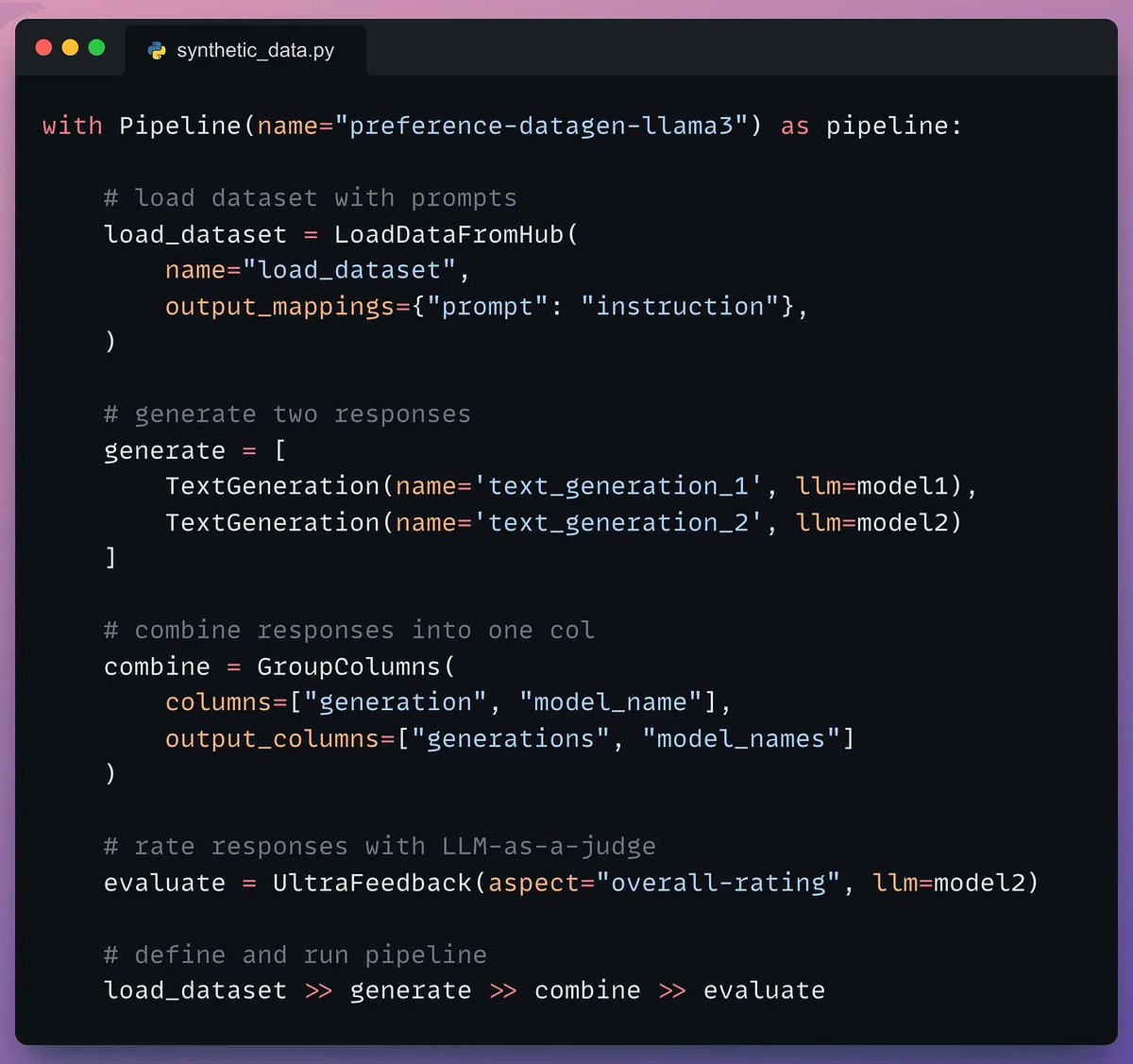
Next, we define our pipeline:

- Load dataset.
- Generate two responses.
- Combine the responses into one column.
- Evaluate the responses with an LLM.
- Define and run the pipeline.

Check this👇

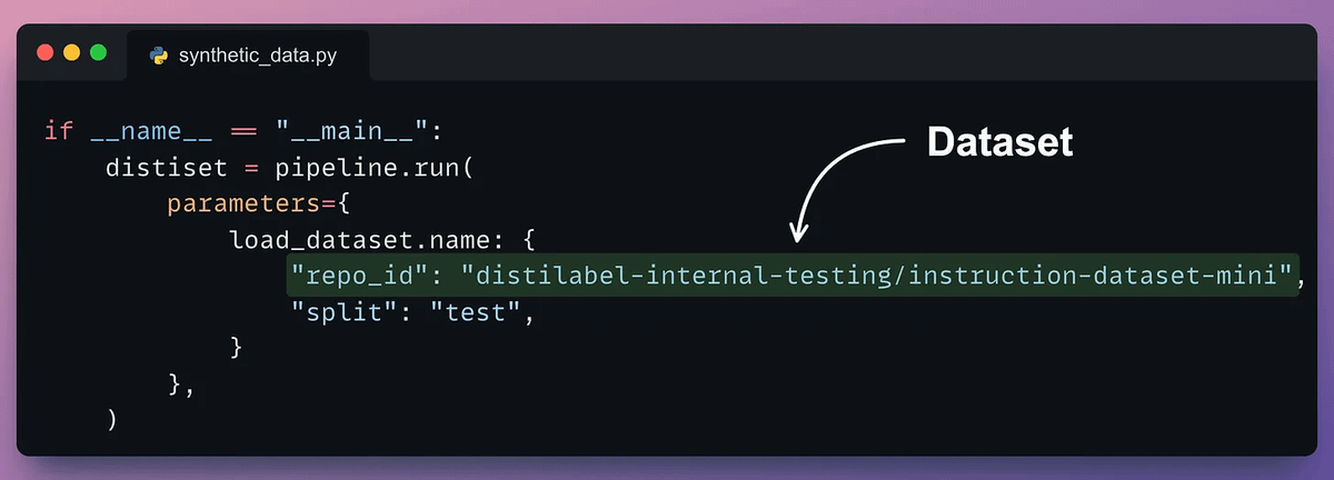
Once the pipeline has been defined, we need to execute it by giving it a seed dataset.

The seed dataset helps it generate new but similar samples.

Check this code👇

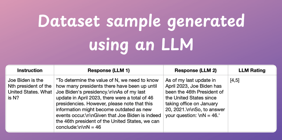
Done!

This produces the instruction and response synthetic dataset as desired.

Check the sample below👇

Here's the instruction fine-tuning process again for your reference.

- Generate responses from two LLMs.
- Rank the response using another LLM.
- Pick the best-rated response and pair it with the instruction.

Check this👇

https://twitter.com/1175166450832687104/status/1947184607277019582

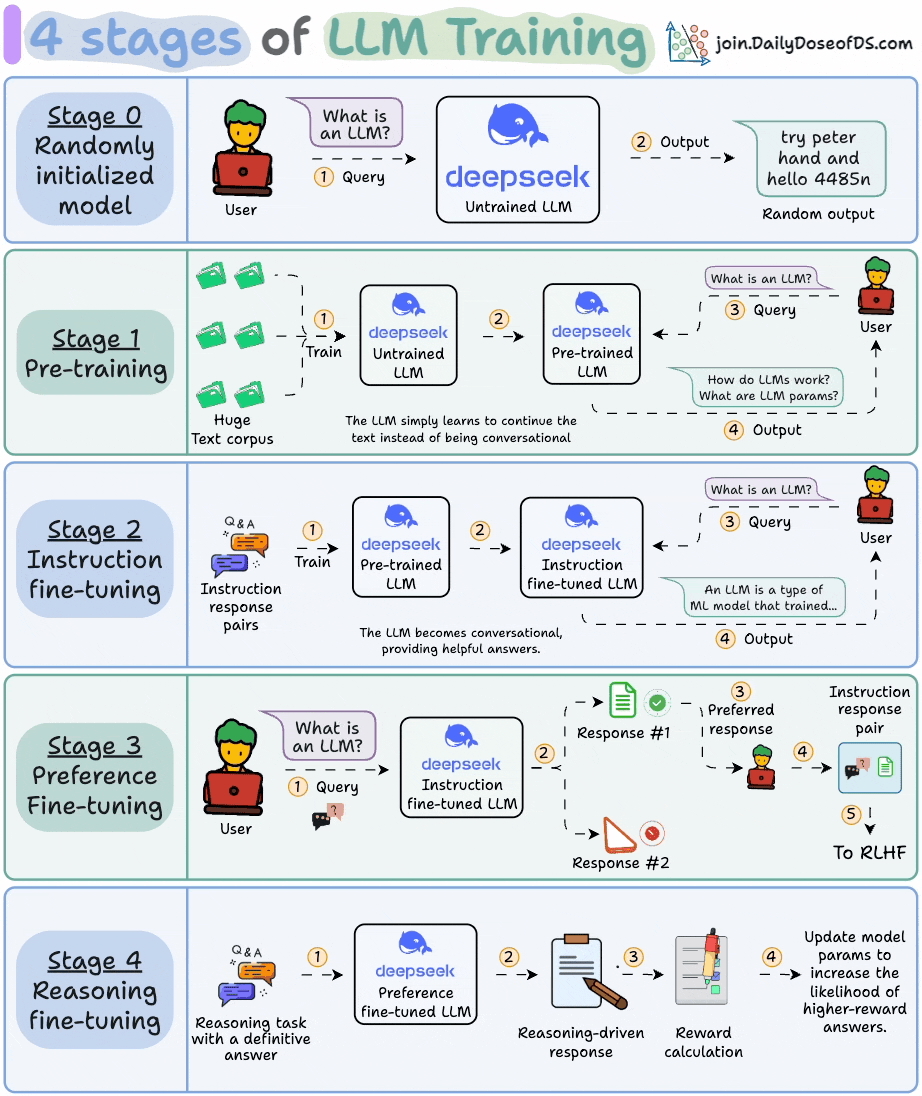
For further reading, I covered the 4 stages of training LLMs from scratch in the thread below.

This visual summarizes what I covered👇

https://twitter.com/1175166450832687104/status/1947184607277019582

https://twitter.com/1175166450832687104/status/1964215272941957367

That's a wrap!

If you found it insightful, reshare it with your network.

Find me → @_avichawla
Every day, I share tutorials and insights on DS, ML, LLMs, and RAGs.

https://twitter.com/1175166450832687104/status/1964215272941957367

• • •

Missing some Tweet in this thread? You can try to force a refresh

This Thread may be Removed Anytime!

Twitter may remove this content at anytime! Save it as PDF for later use!

More from @_avichawla

Avi Chawla

@_avichawla

Jan 22

A simple technique trains neural nets 4-6x faster!

- OpenAI used it in GPT models.
- Meta used it in LLaMA models.
- Google used it in Gemini models.

Here's a breakdown (with code):

Typical deep learning frameworks are conservative when it comes to assigning data types.

The default data type is usually 64-bit or 32-bit, when they could have used 16-bit, for instance.

This is also evident from the code below👇

As a result, we are not entirely optimal at allocating memory.

Of course, this is done to ensure better precision in representing information.

However, this precision comes at the cost of memory utilization, which is not desired in all situations.

Check this 👇

Read 12 tweets

Avi Chawla

@_avichawla

Dec 12, 2025

- Google Maps uses graph ML to predict ETA
- Netflix uses graph ML in recommendation
- Spotify uses graph ML in recommendation
- Pinterest uses graph ML in recommendation

Here are 6 must-know ways for graph feature engineering (with code):

Like images, text, and tabular datasets have features, so do graph datasets.

This means when building models on graph datasets, we can engineer these features to achieve better performance.

Let's discuss some feature engineering techniques below!

First, let’s create a dummy social networking graph dataset with accounts and followers (which will also be accounts).

We create the two DataFrames shown below, an accounts DataFrame and a followers DataFrame.

Check this code👇

Read 14 tweets

Avi Chawla

@_avichawla

Dec 10, 2025

You're in an AI Engineer interview at OpenAI.

The interviewer asks:

"Our GPT model generates 100 tokens in 42 seconds.

How do you make it 5x faster?"

You: "I'll allocate more GPUs for faster generation."

Interview over.

Here's what you missed:

The real bottleneck isn't compute, it's redundant computation.

Without KV caching, your model recalculates keys and values for each token, repeating work.

- with KV caching → 9 seconds
- without KV caching → 42 seconds (~5x slower)

Let's dive in to understand how it works!

To understand KV caching, we must know how LLMs output tokens.

- Transformer produces hidden states for all tokens.
- Hidden states are projected to the vocab space.
- Logits of the last token are used to generate the next token.
- Repeat for subsequent tokens.

Check this👇

Read 10 tweets

Avi Chawla

@_avichawla

Dec 7, 2025

You're in a Research Scientist interview at OpenAI.

The interviewer asks:

"How would you expand the context length of an LLM from 2K to 128K tokens?"

You: "I will fine-tune the model on longer docs with 128K context."

Interview over.

Here's what you missed:

Extending the context window isn't just about larger matrices.

In a traditional transformer, expanding tokens by 8x increases memory needs by 64x due to the quadratic complexity of attention. Refer to the image below!

So, how do we manage it?

continue...👇

1) Sparse Attention

It limits the attention computation to a subset of tokens by:

- Using local attention (tokens attend only to their neighbors).
- Letting the model learn which tokens to focus on.

But this has a trade-off between computational complexity and performance.

Read 12 tweets

Avi Chawla

@_avichawla

Nov 25, 2025

Context engineering, clearly explained (with visuals):

(an illustrated guide below)

So, what is context engineering?

It’s the art and science of delivering the right information, in the right format, at the right time, to your LLM.

Here's a quote by Andrej Karpathy on context engineering...👇

To understand context engineering, it's essential to first understand the meaning of context.

Agents today have evolved into much more than just chatbots.

The graphic below summarizes the 6 types of contexts an agent needs to function properly.

Check this out 👇

Read 10 tweets

Avi Chawla

@_avichawla

Oct 27, 2025

8 key skills to master LLM Engineering:

(free/open-source resources below)

https://twitter.com/_avichawla/status/1974723734503342091

1️⃣ Prompt engineering

Prompt engineering is far from dead!

The key is to craft structured prompts that reduce ambiguity and result in deterministic outputs.

Treat it as engineering, not copywriting!

Here's something I published on JSON prompting:

https://twitter.com/_avichawla/status/1974723734503342091

2️⃣ RAG systems

RAG is 80% retrieval and 20% generation. So if you sort out retrieval, the hard part is over.

Airweave (open-source) lets you build live, bi-temporal knowledge bases so that your LLMs always reason on the freshest facts.

Repo: github.com/airweave-ai/ai…

Supports fully agentic retrieval with semantic and keyword search, query expansion, and more across 30+ sources.