Thread by @keenanisalive

“Everyone knows” what an autoencoder is… but there's an important complementary picture missing from most introductory material.

In short: we emphasize how autoencoders are implemented—but not always what they represent (and some of the implications of that representation).🧵

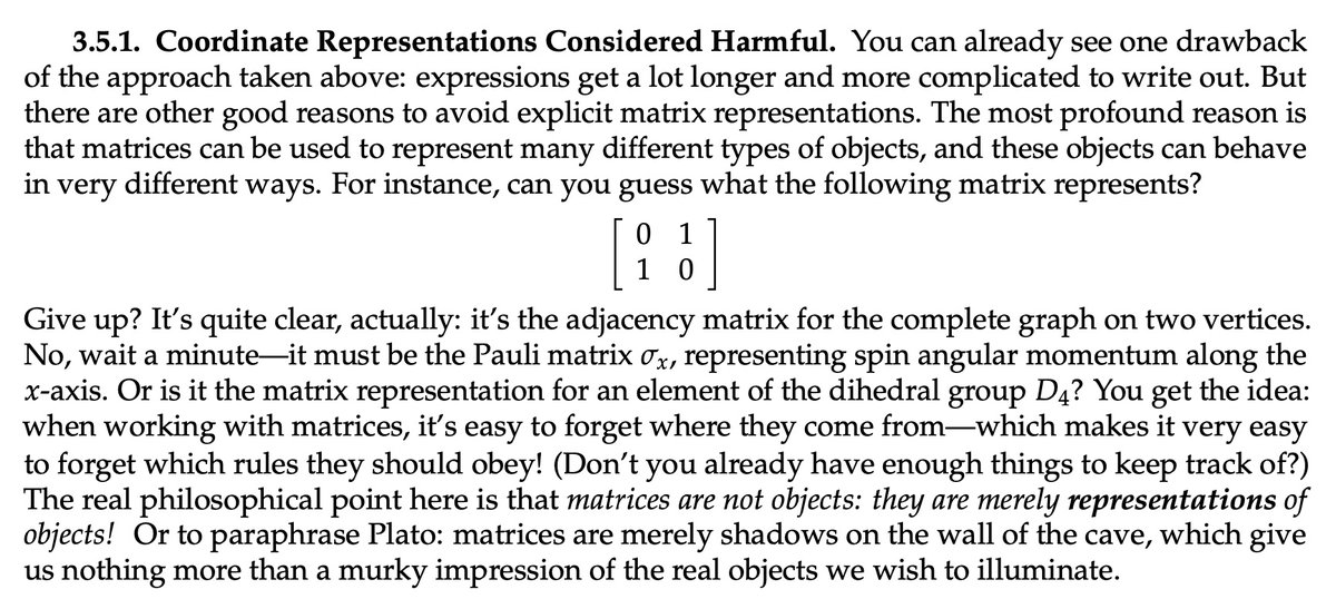
A similar thing happens when (many) people learn linear algebra:

They confuse the representation (matrices) with the objects represented by those matrices (linear maps… or is it a quadratic form?)

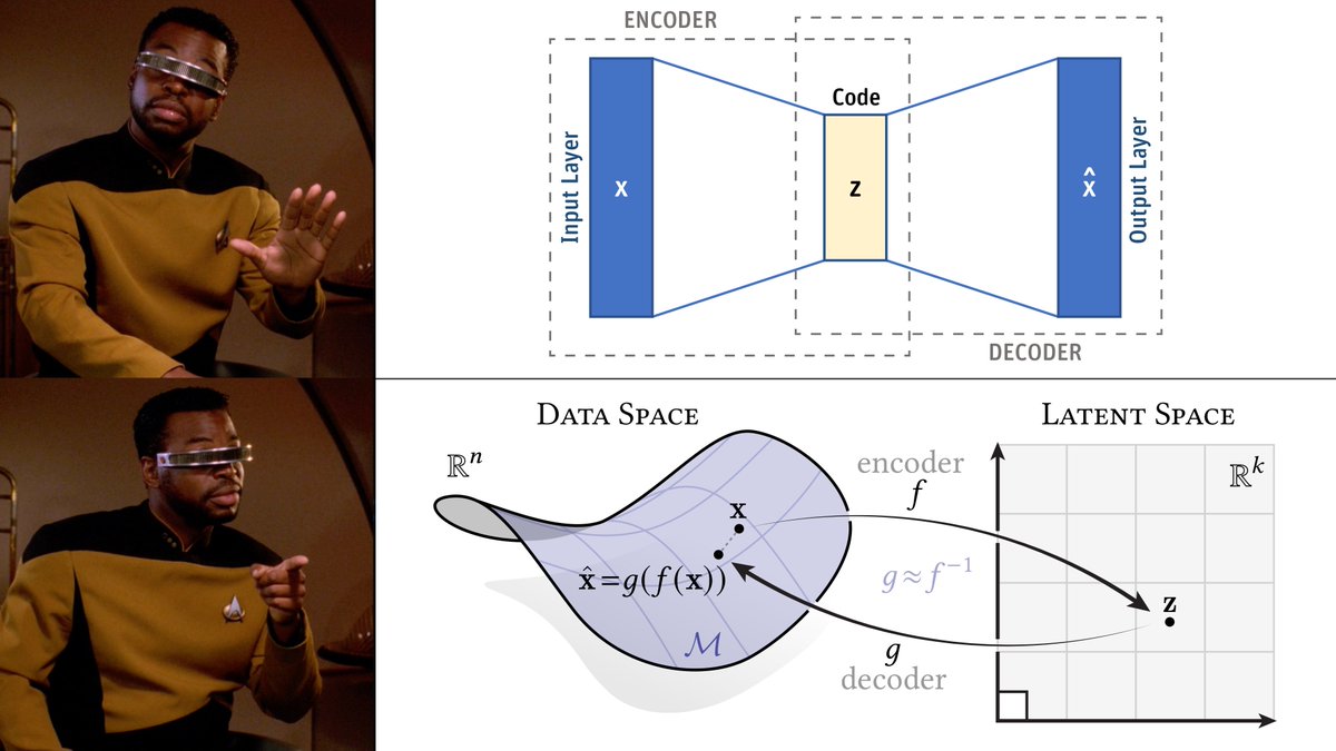
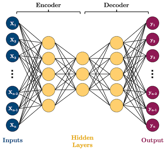
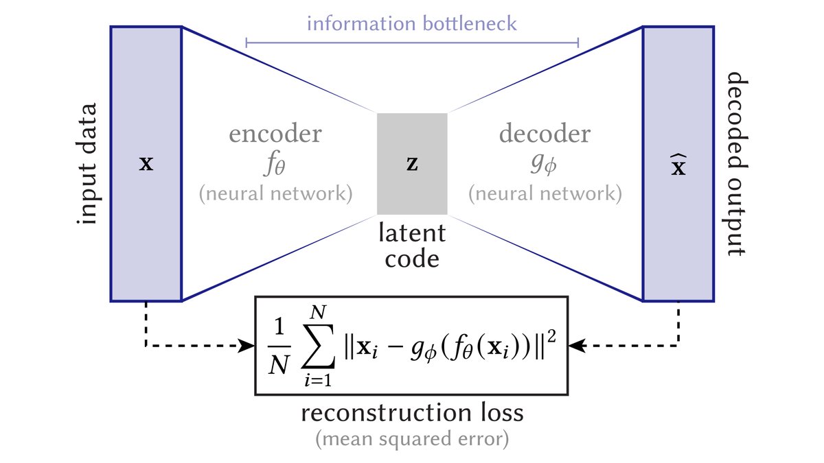
With autoencoders, the first (and last) picture we see often looks like this one: a network architecture diagram, where inputs get “compressed”, then decoded.

If we're lucky, someone bothers to draw arrows that illustrate the main point: we want the output to look like the input!

This picture is great if you want to simply close your eyes and implement something.

But suppose your implementation doesn't work—or you want to squeeze more performance out of your data.

Is there another picture that helps you think about what's going on?

(Obviously: yes!)

Here's a way of visualizing the maps *defined by* an autoencoder.

The encoder f maps high-dimensional data x to low-dimensional latents z. The decoder tries to map z back to x. We *always* learn a k-dimensional submanifold M, which is reliable only where we have many samples z.

In regions where we don't have many samples, the decoder g isn't reliable: we're basically extrapolating (i.e., guessing) what the true data manifold looks like.

The diagram suggests this idea by “cutting off” the manifold—but in reality there’s no clear, hard cutoff.

Another thing made clear by this picture is that, no matter what the true dimension of the data might be, the manifold M predicted by the decoder generically has the same dimension as the latent space: it's the image of R^k under g.

So, the latent dimension is itself a prior.

It should also be clear that, unless the reconstruction loss is exactly zero, the learned manifold M only approximates (rather than interpolates) the given data. For instance, x does not sit on M, even though x̂ does.

(If M does interpolate all xᵢ, you're probably overfitting)

Finally, a natural question raised by this picture is: how do I sample/generate new latents z? For a “vanilla” autoencoder, there's no simple a priori description of the high-density regions.

This situation motivates *variational* autoencoders (which are a whole other story…).

Personally, I find both of these diagrams a little bit crowded—here's a simpler “representation” diagram, with fewer annotations (that might anyway be better explained in accompanying text).

Likewise, here's a simpler “implementation” diagram, that still retains the most important idea of an *auto*-encoder, namely, that you're comparing the output against *itself*.

If you want to use or repurpose these diagrams, the source files (as PDF) can be found at

cs.cmu.edu/~kmcrane/Autoe…

Of course, there will be those who say that the representation diagram is “obvious,” and “that's what everyone has in their head anyway.”

If so… good for you! If not, I hope this alternative picture provides some useful insight as you hack in this space.

[End 🧵]

P.S. I should also mention that these diagrams were significantly improved via feedback from many folks from here and elsewhere.

Hopefully they account for some of the gripes—if not, I'm ready for the next batch! 😉

https://x.com/keenanisalive/status/1961559905850028341