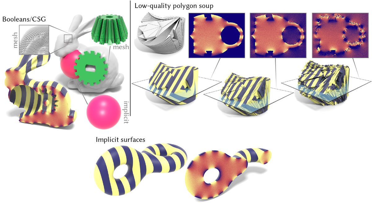
Excited to share a new #SIGGRAPH2021 paper with @markgillesie81 and Boris Springborn that is a pretty big breakthrough in mesh parameterization: cs.cmu.edu/~kmcrane/Proje…
In short: no matter how awful your mesh is, we compute beautiful high-quality texture coordinates.
(1/n)
In short: no matter how awful your mesh is, we compute beautiful high-quality texture coordinates.
(1/n)

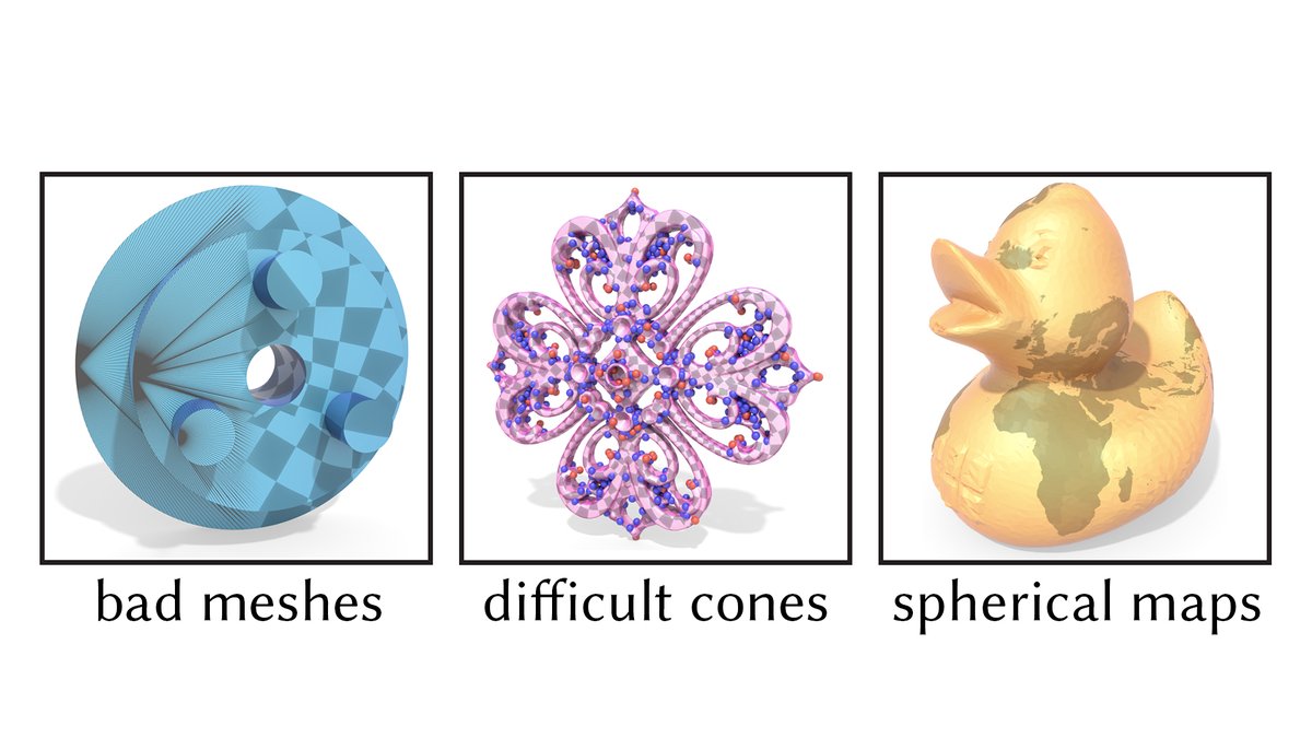
For instance, just as a stress test we can try to flatten this crazy #Thingi10k model as a single piece, rather than cutting it up into many charts. We still get excellent texture coordinates, with no flipped triangles, no angle distortion, and little scale distortion.
(2/n)
(2/n)
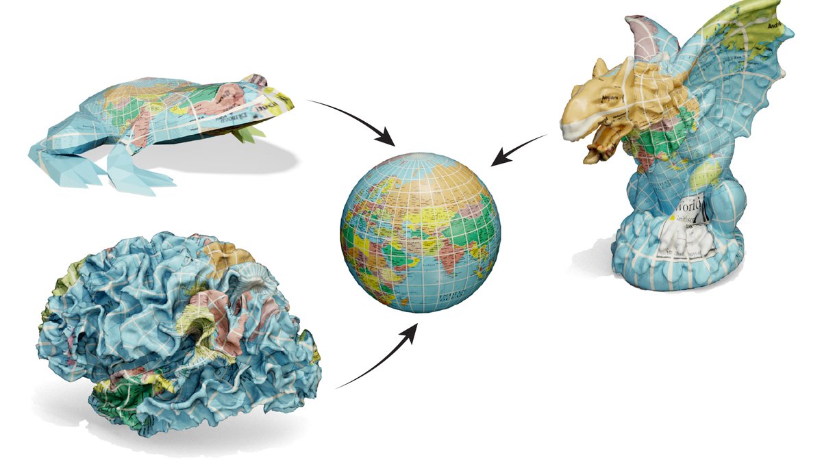
In general, the algorithm is guaranteed to produce maps that do not locally fold over and are perfectly conformal in a discrete sense, for absolutely any triangle mesh. It also gives globally 1-to-1 maps to the sphere, and handles any configuration of "cone singularities" (3/n) 
Our starting point is the "uniformization theorem": any smooth surface—no matter how crazy it looks—can be deformed into a constant-curvature space (e.g. a sphere) by a "conformal" or angle-preserving map
See here for an intro:
(4/n)
See here for an intro:
(4/n)

A recent "discrete uniformization theorem" provides a perfect analog of the smooth one: every polyhedral surface—no matter how crazy it looks—can be mapped to a discretely conformally equivalent one w/ given curvature
Great theorem—but how do you actually compute the map?! (5/n)
Great theorem—but how do you actually compute the map?! (5/n)
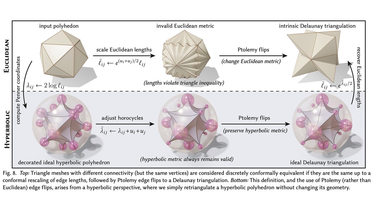
A key idea of the discrete uniformization theorem is to allow the mesh connectivity to change as you flatten the surface. This ensures that you always arrive at a solution—but leads to other challenges that need to be addressed if you want a real, working algorithm. (6/n)
We add three key pieces to ensure things really always work in practice:
A. Improved optimization via "Ptolemy flips" to skirt invalid edge lengths
B. A new integer-based data structure to track how triangulations intersect
C. High-quality interpolation in the "light cone" (7/n)
A. Improved optimization via "Ptolemy flips" to skirt invalid edge lengths
B. A new integer-based data structure to track how triangulations intersect
C. High-quality interpolation in the "light cone" (7/n)
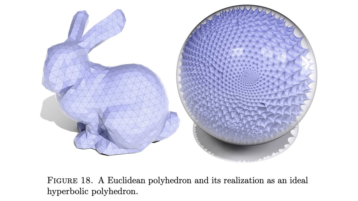
A. One key idea is that every triangle mesh can also be viewed as an "ideal hyperbolic polyhedron." And even if an edge flip yields lengths that violate the triangle inequality, the hyperbolic picture still makes sense! The algorithm can hence continue without any trouble. (8/n) 
B. Another nice idea is that the way two triangulations cross can be recovered from just the *number* of crossings on each edge. We augment these so-called "normal coordinates" (common in topology) with a new mechanism called "roundabouts," needed to recover the final map. (9/n) 

C. Finally, it's not enough to just know how triangulations cross—we must also map data (texture coordinates, color, etc.) back to the input surface. Here, the "light cone" model of hyperbolic geometry helps significantly improve on ordinary piecewise linear interpolation. (10/n) 

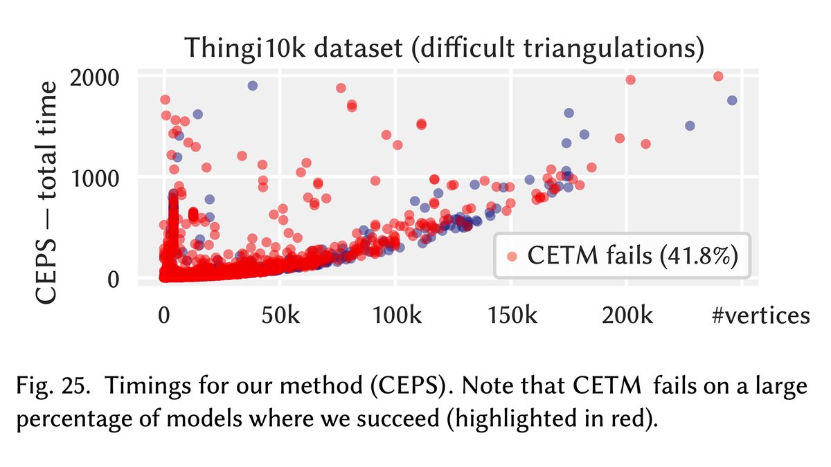
The final algorithm is extremely robust, flattening almost all 32,744 connected components from #Thingi10k—a feat never achieved with prior "guaranteed injective" methods. Yet we guarantee not only injectivity, but also *quality*: all maps are exactly discretely conformal. (11/n) 
There's much more to say here, and the theory runs pretty deep. Here are some good entry points:
@GeometryProcess grad school lecture:
Intro to discrete conformal maps: cs.cmu.edu/~kmcrane/Proje…
Original CETM paper: multires.caltech.edu/pubs/ConfEquiv…
Enjoy! (n/n)
@GeometryProcess grad school lecture:
Intro to discrete conformal maps: cs.cmu.edu/~kmcrane/Proje…
Original CETM paper: multires.caltech.edu/pubs/ConfEquiv…
Enjoy! (n/n)
Thanks to @SaulSchleimer, by the way, for some helpful discussions about/references to normal coordinates. (Forgot to acknowledge you on the webpage, but got it right in the paper!)
• • •
Missing some Tweet in this thread? You can try to
force a refresh

