Thread by @haltakov

Machine Learning Formulas Explained! 👨‍🏫

This is the formula for the Binary Cross Entropy Loss. It is commonly used for binary classification problems.

It may look super confusing, but I promise you that it is actually quite simple!

Let's go step by step 👇

#RepostFriday

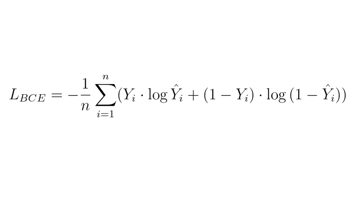
The Cross-Entropy Loss function is one of the most used losses for classification problems. It tells us how well a machine learning model classifies a dataset compared to the ground truth labels.

The Binary Cross-Entropy Loss is a special case when we have only 2 classes.

👇

The most important part to understand is this one - this is the core of the whole formula!

Here, Y denotes the ground-truth label, while Ŷ is the predicted probability of the classifier.

Let's look at a simple example before we talk about the logarithm... 👇

Imagine we have a bunch of photos and we want to classify each one as being a photo of a bird or not.

All photos are manually so that Y=1 for all bird photos and Y=0 for the rest.

The classifier (say a NN) outputs a probability of the photo containing a bird, like Ŷ=0.9

👇

Now, let's look a the logarithm.

Since Ŷ is a number between 0 and 1, log Ŷ will be a negative number increasing up to 0.

Let's take an example of a bird photo (Y=1):
▪️ Classifier predicts 99% bird, so we get -0.01
▪️ Classifier predicts 5% bird, so we get -3

That's weird 👇

For a loss, we want a value close to 0 if the classifier is right and a large value when the classifier is wrong. In the example above it was the opposite!

Fortunately, this is easy to fix - we just need to multiply the value by -1 and can interpret the value as an error 🤷‍♂️

👇

If the photo is labeled as no being a bird, then we have Y=0 and so the whole term becomes 0.

That's why we have the second part - the negative case. Here we just take 1-Y and 1-Ŷ for the probabilities. We are interested in the probability of the photo not being a bird.

👇

Combining both we get the error for one data sample (one photo). Note that one of the terms will always be 0, depending on how the photo is labeled.

This is actually the case if we have more than 2 classes as well when using one-hot encoding!

OK, almost done with that part 👇

Now, you should have a feeling of how the core of the formula works, but why do we use a logarithm?

I won't go into detail, but let's just say this is a common way to formulate optimization problems in math - the logarithm makes all multiplications to sums.

Now the rest 👇

We know how to compute the loss for one sample, so now we just take the mean over all samples in our dataset (or minibatch) to compute the loss.

Remember - we need to multiply everything by -1 so that we can invert the value and interpret it as a loss (low good, high bad).

👇

Where to find it in your ML framework?

The Cross-Entropy Loss is sometimes also called Log Loss or Negative Log Loss.

▪️ PyTorch - torch.nn.NLLLoss
▪️ TensorFlow - tf.keras.losses.BinaryCrossentropy and CategoricalCrossentropy
▪️ Scikit-learn - sklearn.metrics.log_loss

And if it is easier for you to read code than formulas, here is a simple implementation and two examples of a good (low loss) and a bad classifier (high loss).

Every Friday I repost one of my old threads so more people get the chance to see them. During the rest of the week, I post new content on machine learning and web3.

If you are interested in seeing more, follow me @haltakov