Thread by @selcukorkmaz

1/ 🤔 Ever wonder how "bootstrapping" works? I recently used it for estimating confidence intervals & someone asked me about its logic. At first, I was stumped, even though I've used it often! Here's my attempt to clarify.

#Statistics #Bootstrapping #DataScience 📈📉

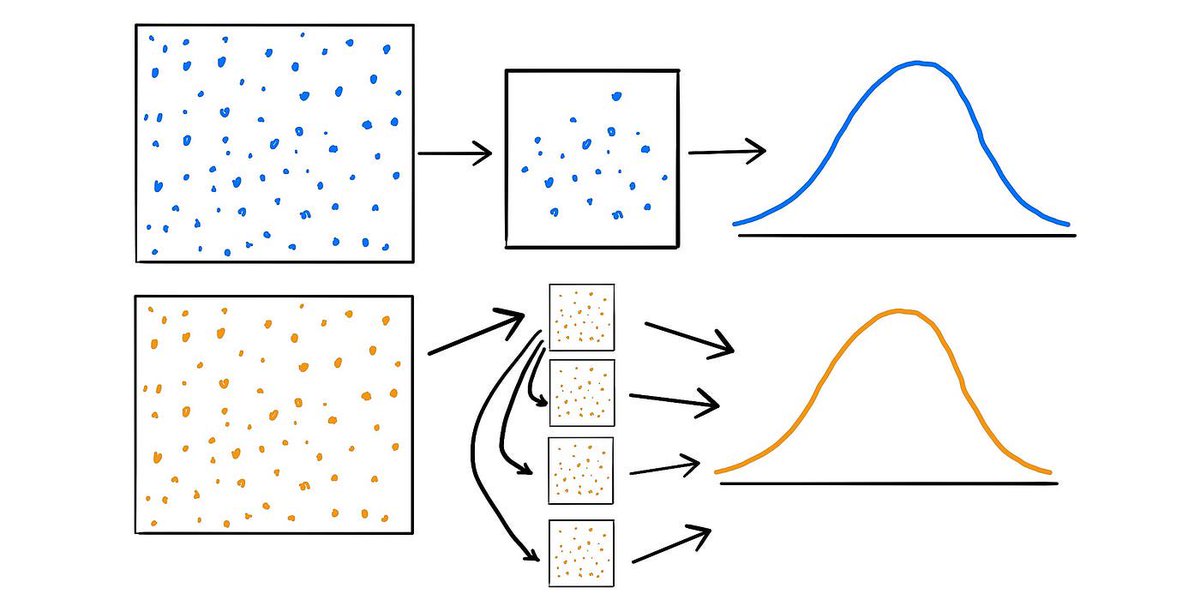
2/ 🥾 What's bootstrapping? It's a resampling technique where you take many subsamples from your sample data & analyze them. The idea? The subsamples give us an insight into the variability in our sample.

3/ 🤷‍♂️ But how do we go from understanding our sample to drawing conclusions about a larger population? Here’s the tricky part. The underlying assumption is that our sample is a good representation of the population.

4/ 💡 If the original sample is representative, resampling from it mimics drawing multiple samples from the population. By assessing the variability across bootstrapped samples, we infer the population's variability.

5/ 🎯 Remember, statistics is about estimation. With bootstrapping, we're creating a distribution of estimates. This distribution helps us understand how stable or variable our original estimate might be.

6/ 🔄 Think of it as a simulated "what if" scenario. What if we took many samples from the population? Bootstrapping replicates that process by resampling from our best available representation of the population - our sample!

7/ ⚠️ But there are limitations. If your initial sample is biased or unrepresentative, bootstrapping can't fix that. It can only provide information based on the data you have. Hence, ensuring a good sample is crucial.

8/ 🔍 Also, bootstrapping isn't a silver bullet for every statistical scenario. But it's especially useful when the sample size is small or when the underlying distribution is unknown.

9/ 🌟 So, the leap from understanding our sample to making inferences about the population using bootstrapping is rooted in the idea that by understanding variability in our sample, we get a window into variability in the larger population.

10/ 🚀 In essence, bootstrapping takes our single sample & amplifies its insights, giving us a richer perspective. It’s a powerful tool in our statistical arsenal, as long as we remember its assumptions & limitations.