There is a common misconception that all probability distributions are like a Gaussian.

Often, the reasoning involves the Central Limit Theorem.

This is not exactly right: they resemble Gaussian only from a certain perspective.

🧵 👇🏽
Let's state the CLT first. If we have 𝑋₁, 𝑋₂, ..., 𝑋ₙ independent and identically distributed random variables, their scaled sum is a Gaussian distribution in the limit.

The surprising thing here is the limit is independent of the variables' distribution.
Note that the random variables undergo a significant transformation: averaging and scaling with the mean, the variance, and √𝑛.

(The scaling transformation is the "certain perspective" I mentioned in the first tweet.)
How can we unravel what this transformation means?

For this, we have to go back to the Law of Large Numbers, which states that the average converges to the expected value.

The Central Limit Theorem is essentially the speed of this convergence!

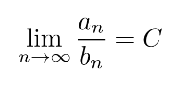
In general, if we have two sequences of numbers 𝑎ₙ and 𝑏ₙ, we can compare their magnitudes by taking the limit of their ratio.

When both 𝑎ₙ and 𝑏ₙ converges to 0, the existence of this limit implies that they have the same speed.
In the Central Limit Theorem, we essentially take the ratio of two such sequences, as you can see below.
When we write out the limit, we immediately see why.
Since we are talking about random variables and not deterministic sequences, the situation is a bit more complicated.

In the Central Limit Theorem, the convergence is in distribution, not in a pointwise sense. (Keep in mind that random variables are functions.)
The fact that the limiting distribution is a Gaussian means that we not only know the rate of convergence of the scaled averages, we also know how much it fluctuates around the sequence we compare it to.

(Which is 1/√𝑛.)
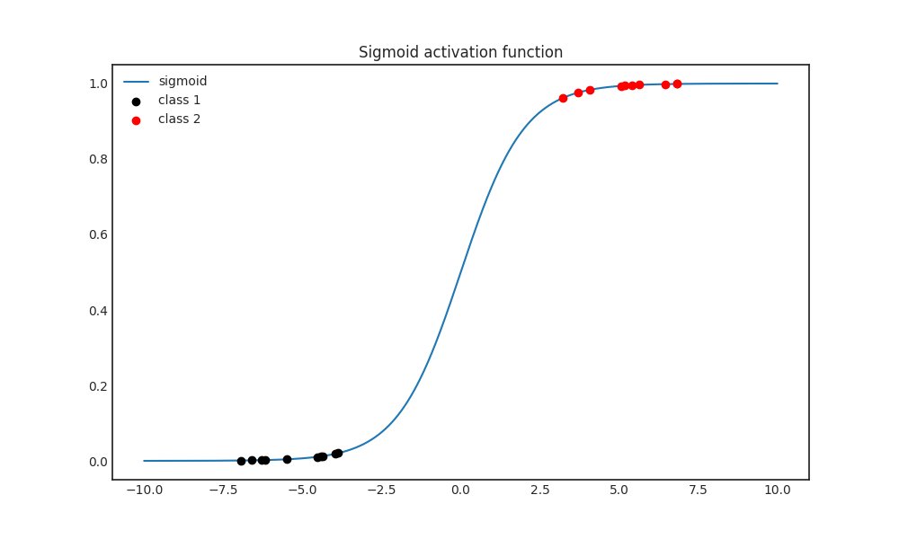
To summarize, a real-life distribution only resembles a Gaussian if it is an average of independent measurements.

A good example is the winnings of a poker player, averaged per hand.
A famous, not Gaussian-like distribution is the Pareto distribution. This often captures the phenomenon where the vast majority of samples have low value and a minority is extremely high.

Wealth distribution and the number of Facebook friends both fall into this category.
TL;DR: not all distributions are Gaussian. Only their properly scaled averages are, if they are independent and identically distributed with finite mean and variance.

• • •

Missing some Tweet in this thread? You can try to force a refresh
 

Keep Current with Tivadar Danka

Tivadar Danka Profile picture

Stay in touch and get notified when new unrolls are available from this author!

Read all threads

This Thread may be Removed Anytime!

PDF

Twitter may remove this content at anytime! Save it as PDF for later use!

Try unrolling a thread yourself!

how to unroll video
  1. Follow @ThreadReaderApp to mention us!

  2. From a Twitter thread mention us with a keyword "unroll"
@threadreaderapp unroll

Practice here first or read more on our help page!

More from @TivadarDanka

8 Apr
One of my favorite convolutional network architectures is the U-Net.

It solves a hard problem in such an elegant way that it became one of the most performant and popular choices for semantic segmentation tasks.

How does it work?

🧵 👇🏽
Let's quickly recap what semantic segmentation is: a common computer vision task, where we want to classify which class each pixel belongs to.

Because we want to provide a prediction on a pixel level, this task is much harder than classification.
Since the absolutely classic paper Fully Convolutional Networks for Semantic Segmentation by Jonathan Long, Evan Shelhamer, and Trevor Darrell, fully end-to-end autoencoder architectures were most commonly used for this.

(Image source: paper above, arxiv.org/abs/1411.4038v2) Image
Read 10 tweets
1 Apr
Gradient descent sounds good on paper, but there is a big issue in practice.

For complex functions like training losses for neural networks, calculating the gradient is computationally very expensive.

What makes it possible? For one, stochastic gradient descent!

🧵 👇🏽
When you have a lot of data, calculating the gradient of the loss involves the computation of a large sum.

Think about it: if 𝑥ᵢ denotes the data and 𝑤 denotes the weights, the loss function takes the form below.
Not only do we have to add a bunch of numbers together, but we have to find the gradient of each loss term.

For example, if the model contains 10 000 parameters and 1 000 000 data points, we need to compute 10 000 x 1 000 000 = 10¹⁰ derivatives.

This can take a LOT of time.
Read 7 tweets
31 Mar
Gradient descent has a really simple and intuitive explanation.

The algorithm is easy to understand once you realize that it is basically hill climbing with a really simple strategy.

Let's see how it works!

🧵 👇🏽
For functions of one variable, the gradient is simply the derivative of the function.

The derivative expresses the slope of the function's tangent plane, but it can also be viewed as a one-dimensional vector!
When the function is increasing, the derivative is positive. When decreasing, it is negative.

Translating this to the language of vectors, it means that the "gradient" points to the direction of the increase!

This is the key to understand gradient descent.
Read 9 tweets
27 Mar
Sigmoid is one of most commonly used activation functions.

However, it has a serious weakness: Sigmoids often make the gradient disappear.

This can leave the network stuck during training, so they effectively stop learning.

How can this happen?

🧵 👇🏽
Let's take a look at the Sigmoid function first.

Notice below that as 𝑥 tends to ∞ or -∞, the function flattens out.

This can happen for instance when the previous layer separates the classes very well, mapping them far away from each other in the feature space.
Why is this a problem?

Flatness means that the derivative is close to zero, as shown in the figure below.
Read 7 tweets
22 Mar
What if you want to optimize a function, but every evaluation costs you $100 and takes a day to execute?

Algorithms like gradient descent build on two key assumptions:

• function is differentiable,
• and you can calculate it on demand.

What if this is not the case?

🧵 👇🏽
For example, you want to tune the hyperparameters of a model that requires 24 hours of GPU time to train.

Can you find a good enough value under reasonable time and budget?

One method is the so-called Bayesian optimization.
Essentially, the method works as follows.

1️⃣ Model the expensive function with a Gaussian process.

Gaussian processes are easy to compute and offer a way to quantify uncertainty in the predictions.
Read 14 tweets
15 Mar
Building a good training dataset is harder than you think.

For example, you can have millions of unlabelled data points, but only have the resources to label a thousand.

This is a story is about a case that I used to encounter almost every day in my work.

🧵 👇🏽
Do you know how new drugs are developed?

Essentially, thousands of candidate molecules are tested to see if they have the targeted effect. First, the testing is done on cell cultures.

Sometimes, there is no better option than scanning through libraries of molecules.
After cells are treated with a given molecule (or molecules in some cases), the effects are studied by screening them with microscopy.

The treated cells can exhibit hundreds of different phenotypes ( = classes), some of them might be very rare.
Read 12 tweets

Did Thread Reader help you today?

Support us! We are indie developers!


This site is made by just two indie developers on a laptop doing marketing, support and development! Read more about the story.

Become a Premium Member ($3/month or $30/year) and get exclusive features!

Become Premium

Too expensive? Make a small donation by buying us coffee ($5) or help with server cost ($10)

Donate via Paypal Become our Patreon

Thank you for your support!

Follow Us on Twitter!