Thread by @TivadarDanka

What you see below is a 2D representation of the MNIST dataset.

It was produced by t-SNE, a completely unsupervised algorithm. The labels were unknown to it, yet it almost perfectly separates the classes. The result is amazing.

This is how the magic is done!

🧵 👇🏽

Even though real-life datasets can have several thousand features, often the data itself lies on a lower-dimensional manifold.

Dimensionality reduction aims to find these manifolds to simplify data processing down the line.

So, we have data points 𝑥ᵢ in a high-dimensional space, looking for lower dimensional representations 𝑦ᵢ.

We want the 𝑦ᵢ-s to preserve as many properties of the original as possible.

For instance, if 𝑥ᵢ is close to 𝑥ⱼ, we want 𝑦ᵢ to be close to 𝑦ⱼ as well.

The t-Distributed Stochastic Neighbor Embedding algorithm (t-SNE) achieves this by modeling the dataset with a dimension-agnostic probability distribution, finding a lower-dimensional approximation with a closely matching distribution.

Let's unravel this a bit.

Since we want to capture an underlying cluster structure, we define a probability distribution on the 𝑥ᵢ-s that reflects this.

For each data point 𝑥ⱼ, we model the probability of 𝑥ᵢ belonging to the same class ("being neighbors") with the formula below.

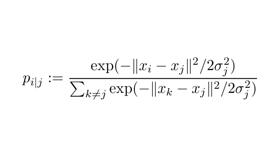
Essentially, we model each point's neighbors with a Gaussian distribution.

The variance σⱼ is a parameter that is essentially given as an input.

We don't set this directly. Instead we specify the expected number of neighbors, called perplexity.

To make the optimization easier, these probabilities are symmetrized. With these symmetric probabilities, we form the distribution 𝑃.

This represents our high-dimensional data.

Similarly, we define a distribution for the 𝑦ᵢ-s, our (soon to be identified) lower-dimensional representation. This distribution is denoted with 𝑄.

Here, we model the "neighborhood-relation" with the Student t-distribution.

This is where the t in t-SNE comes from.

Our goal is to find the 𝑦ᵢ-s through optimization such that 𝑃 and 𝑄 are as close together as possible. (In a distributional sense.)

This closeness is expressed with the Kullback-Leibler divergence.

We have successfully formulated the dimensionality reduction problem as optimization!

From here, we just calculate the gradient of KL divergence with respect to the 𝑦ᵢ-s and find an optimum with gradient descent.

The results are something like below, where you can see t-SNE's output on the MNIST handwritten digits dataset.

I have already shown this at the beginning of the thread. Now you understand how it was made.

This is one of the most powerful illustrations in machine learning.

Interactive visualizations and learning resources!

1) If you want to explore how the t-SNE works on MNIST, here is a little app where you can play around with the 3D point cloud generated by it.

dash-gallery.plotly.host/dash-tsne/

2) t-SNE has several caveats, which are far from obvious. To use it successfully, one must need to be aware of the details and the potential pitfalls.

This awesome publication in @distillpub can help you understand how to use the method effectively.

distill.pub/2016/misread-t…

3) You should also read the original paper "Visualizing High-Dimensional Data Using t-SNE" by Laurens van der Maaten and Geoffrey Hinton. This is where the method was first introduced.

You can find it here: jmlr.org/papers/volume9…

If you enjoyed this explanation, consider following me and hitting a like/retweet on the first tweet of the thread!

I regularly post simple explanations of mathematical concepts in machine learning, make sure you don't miss out on the next one!

https://twitter.com/TivadarDanka/status/1392471126996099073