Read through these awesome notes by @chipro and noticed something interesting about distribution shifts: they form a lattice, so you can represent them like you do sets, ie using a Venn diagram!
I find this view super helpful for understanding shifts, so let's walk through it.
I find this view super helpful for understanding shifts, so let's walk through it.
https://twitter.com/chipro/status/1490924046350909442

(inb4 pedantry: the above diagram is an Euler diagram, not a Venn diagram, meaning not all possible joins are represented. that is good, actually, for reasons to be revealed!)
From the notes: joint distribution of data X and targets Y is shifting. We can decompose the joint into two pieces (marginal and conditional) in two separate ways (from Y or X).
There are four major classes of distribution shift, defined by which pieces vary and which don't.
There are four major classes of distribution shift, defined by which pieces vary and which don't.

Wait, you say, where's the fourth shift?
Because of price increases due to global supply chain issues, we can only afford 3 distribution shifts in this post, where there should be 4.
Because of price increases due to global supply chain issues, we can only afford 3 distribution shifts in this post, where there should be 4.
Actually, it just doesn't have a canonical name, because it's "too difficult to study" -- perhaps because it involves the opposite conditional, P(X|Y), from what the model learns, P(Y|X)?
In any case, I'll call it "mechanism drift".
In any case, I'll call it "mechanism drift".

Etymology: if we think of our labels Y as latent variables in a generative model, X|Y is the generative process. Ideally, there's an intervening causal mechanism (dogs cause patterns of light on camera sensors, sentiments cause sentences), which is what has changed in this case.
At first, these four types seem independent -- I have a label shift problem or a covariate shift problem, but not both.
But that's not the case! We can have covariate shift with or without label shift. Read the attached if you want an example.
But that's not the case! We can have covariate shift with or without label shift. Read the attached if you want an example.

This gave me pause, because I realized my intuition was based on only one type of shift happening at a time!
So I dug a little deeper.
So I dug a little deeper.
Fundamentally, this is because Bayes' rule says that
P(Y|X) P(X) = P(X|Y) P(Y)
And if we vary just one term on one side, at least one of the other two terms must vary to compensate.
So distribution shifts are always entangled with each other!
P(Y|X) P(X) = P(X|Y) P(Y)
And if we vary just one term on one side, at least one of the other two terms must vary to compensate.
So distribution shifts are always entangled with each other!
We can choose to vary or not vary each term in this equation, effectively fixing some subset of the distributions while the others change.
So we can relate our distribution shift types to subsets of {Y|X, X, X|Y, Y}.
So we can relate our distribution shift types to subsets of {Y|X, X, X|Y, Y}.
A power set, the set of all subsets, has nice structure.
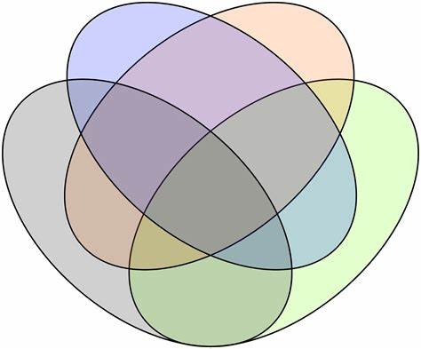
You may have seen that structure depicted geometrically, via Venn diagrams (right), or graphically, via Hasse diagrams (left).

You may have seen that structure depicted geometrically, via Venn diagrams (right), or graphically, via Hasse diagrams (left).


But as noted, Bayes' rule limits what changes we're allowed to make! For example, we can't just change P(Y), because then the RHS of Bayes wouldn't equal the LHS. So there's no such thing as, say, "just the labels changing".
There's also two more disallowed cases: say that P(X) and P(Y|X) both shift, but P(Y) and P(X|Y) are fixed. The latter means the joint P(X,Y) can't change, so the changes must've canceled each other out. So there'd be no shift!
That means we can get away with a diagram that's missing those spots.
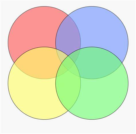
And in fact, there's a common "Venn diagram" that is missing two combinations. This one, where circles on opposite corners do not touch:
And in fact, there's a common "Venn diagram" that is missing two combinations. This one, where circles on opposite corners do not touch:

(legally, this is not a Venn diagram, because a Venn diagram, according to some "official" definitions, must represent all possible combinations, like a power set. but no one knows what an "Euler diagram" is, so chalk this one up to another L for prescriptivist pedants)
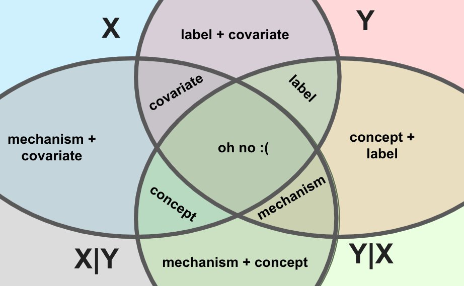
Let's write down this "Venn" diagram with possible choices of distributions to vary while holding the others fixed. 

If we label our diagram with the shift types, we reveal an interesting structure for our four classes of distribution shift: not all pairs can occur together (e.g. no covariate + concept shift) and any triple just results in one type "winning out". 

There's no "ordering" of the shifts based on the triples, btw. Label beats covariate if you add in concept, but covariate beats label if you add in mechanism.
Instead, there's a ring:
covariate <-> label <-> concept <-> mechanism <-> covariate
Instead, there's a ring:
covariate <-> label <-> concept <-> mechanism <-> covariate
So what are the take-homes?
First, I think this diagram and the "power set" view behind it helps clarify what these drifts are: aggregates!
E.g. in the general case, label shift is when concept drift and covariate shift happen together in the absence of mechanism drift.
First, I think this diagram and the "power set" view behind it helps clarify what these drifts are: aggregates!
E.g. in the general case, label shift is when concept drift and covariate shift happen together in the absence of mechanism drift.
(and if label shift isn't accompanied by both, it's accompanied by one or the other! and mutatis mutandis for all the other shifts, based on adjacency in the ring from two tweets ago)
Second, I think it suggests some missing pieces in our distribution shift toolkit.
Can we build specific tools for when shifts happen together? Can we leverage the fact that, say, we know X and Y are both shifting, leaving the conditionals intact, and use a special approach?
Can we build specific tools for when shifts happen together? Can we leverage the fact that, say, we know X and Y are both shifting, leaving the conditionals intact, and use a special approach?
(or maybe those exist already, would love to know if so!)
Finally, I think it clarifies that the unloved fourth shift type, "mechanism drift", is important and worthy of study.
It's hard to study in general, but what if we know it's happening at the same time as covariate shift, so the true discriminative function isn't changing?
It's hard to study in general, but what if we know it's happening at the same time as covariate shift, so the true discriminative function isn't changing?
PS: mechanism + concept is truly terrifying.
The generative model and the discriminative function are both changing, and so is the joint, so the loss is changing (going up, probably).
But the marginals are fixed!
So the shift would only show up if you checked the joint 😬
The generative model and the discriminative function are both changing, and so is the joint, so the loss is changing (going up, probably).
But the marginals are fixed!
So the shift would only show up if you checked the joint 😬
• • •
Missing some Tweet in this thread? You can try to
force a refresh


