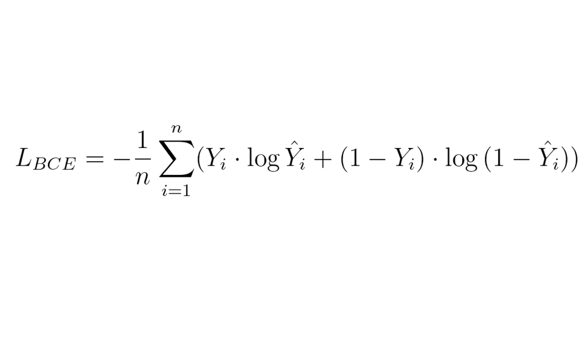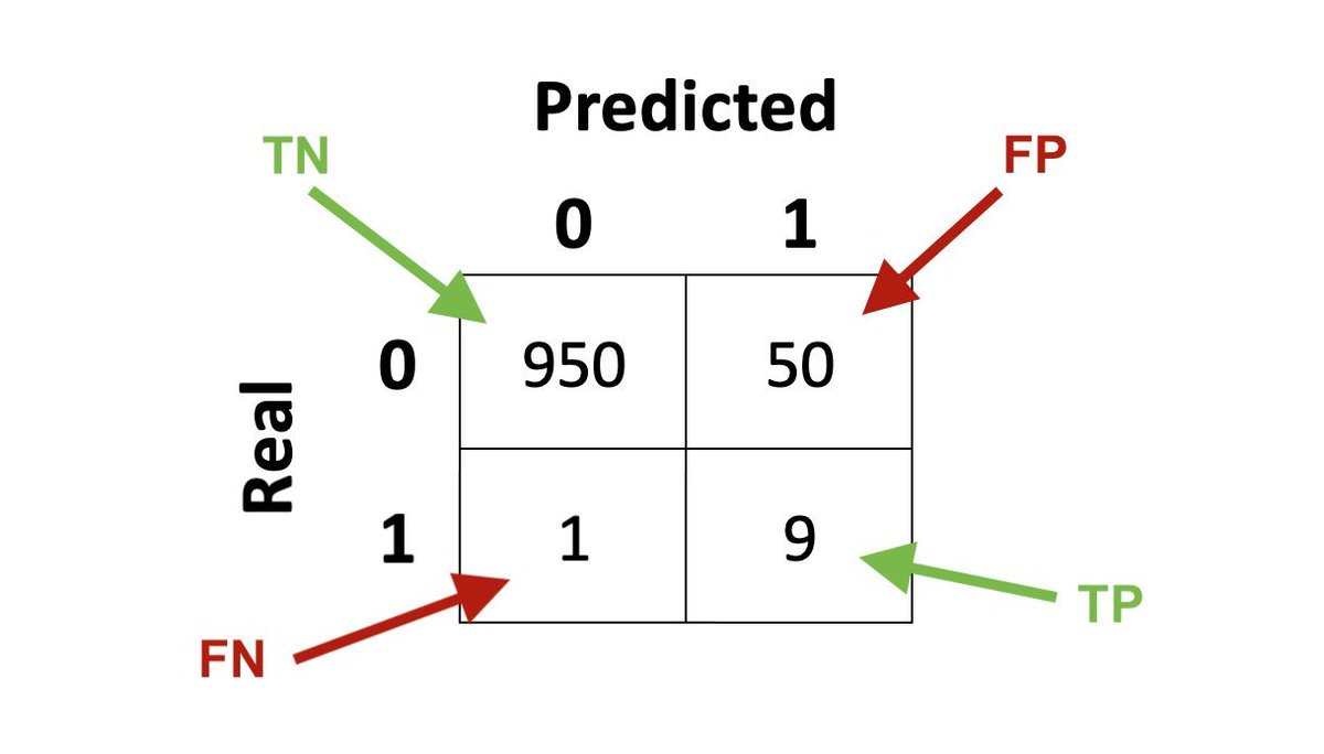
Machine Learning Formulas Explained 👨🏫
This is the Huber loss - another complicated-looking formula...
Yet again, if you break it down and understand the individual, it becomes really easy.
Let me show you 👇
This is the Huber loss - another complicated-looking formula...
Yet again, if you break it down and understand the individual, it becomes really easy.
Let me show you 👇

Background
The Huber loss is a loss function that is similar to the Mean Squared Error (MSE) but it is designed to be more robust to outliers.
MSE suffers from the problem that if there is a small number of severe outliers they can dominate the whole loss
How does it work? 👇
The Huber loss is a loss function that is similar to the Mean Squared Error (MSE) but it is designed to be more robust to outliers.
MSE suffers from the problem that if there is a small number of severe outliers they can dominate the whole loss
How does it work? 👇
The key to understanding math formulas is not to try to understand everything at the same time.
Try looking at the terms inside the formula. Try to understand them from the inside to the outside...
Here, we can quickly see that one term is repeated several times...
👇
Try looking at the terms inside the formula. Try to understand them from the inside to the outside...
Here, we can quickly see that one term is repeated several times...
👇

Here y is the ground truth value we compare to and f(x) is the result provided by our model.
You can think for example about estimating house prices. Then y is the real prices and f(x) is the price our machine learning model predicted.
We can then simplify the formula a bit 👇
You can think for example about estimating house prices. Then y is the real prices and f(x) is the price our machine learning model predicted.
We can then simplify the formula a bit 👇

The next thing we see is that the formula has two parts.
The first part is a simple quadratic term α^2 (with a constant of 0.5).
The second part is a bit convoluted with a couple of constants, but it is an absolute (linear) term - |α|.
Let's simplify further...
The first part is a simple quadratic term α^2 (with a constant of 0.5).
The second part is a bit convoluted with a couple of constants, but it is an absolute (linear) term - |α|.
Let's simplify further...

The parameter δ determines when we choose one part and when the other. Let's try to set to a fixed value for now, so that we can simplify things. Setting δ = 1 gives us the simplest form.
OK, now if you ignore the constants (I'll come back to them later), it is quite simple
👇
OK, now if you ignore the constants (I'll come back to them later), it is quite simple
👇

What the formula now tells us is that we take the square of α close to 0 and the absolute value otherwise.
Let's quickly implement the function in Python and plot it for δ = 1.
Take a look at the plot - do you see the quadratic and the linear part?
👇

Let's quickly implement the function in Python and plot it for δ = 1.
Take a look at the plot - do you see the quadratic and the linear part?
👇


Alright, let me annotate the image a little bit.
You can clearly see how the Huber loss behaves like a quadratic function close to 0 and like the absolute value further away.
OK, now we understand the core of the formula. Let's go back and undo the simplifications...
👇
You can clearly see how the Huber loss behaves like a quadratic function close to 0 and like the absolute value further away.
OK, now we understand the core of the formula. Let's go back and undo the simplifications...
👇

First, what's with these deltas?
We want our loss function to be continuous, so at the border between the two parts (when α = δ) they need to have the same value.
What the constants in the linear term do is just make sure that it equals the quadratic term when α = δ!
👇
We want our loss function to be continuous, so at the border between the two parts (when α = δ) they need to have the same value.
What the constants in the linear term do is just make sure that it equals the quadratic term when α = δ!
👇

Finally, why is this constant 0.5 everywhere? Do we really need it?
The thing is that we typically use a loss function to compute its derivative and optimize our weights. And the derivative of 0.5*α^2 is... simply α.
We use the 0.5 just to make the derivative simpler 🤷♂️
👇
The thing is that we typically use a loss function to compute its derivative and optimize our weights. And the derivative of 0.5*α^2 is... simply α.
We use the 0.5 just to make the derivative simpler 🤷♂️
👇
And if you want to use the Huber loss, you probably don't need to implement it yourself - popular ML libraries already have it implemented:
▪️ PyTorch: torch.nn.HuberLoss
▪️ TensorFlow: tf.keras.losses.Huber
▪️scikit-learn: sklearn.linear_model.HuberRegressor
▪️ PyTorch: torch.nn.HuberLoss
▪️ TensorFlow: tf.keras.losses.Huber
▪️scikit-learn: sklearn.linear_model.HuberRegressor
Summary
The Huber loss takes the form of a quadratic function (like MSE) close to 0 and of a linear function (like MAE) away from zero. This makes it more robust to outliers while keeping it smooth around 0. You control the balance with the parameter δ.
Simple, right? 😁
The Huber loss takes the form of a quadratic function (like MSE) close to 0 and of a linear function (like MAE) away from zero. This makes it more robust to outliers while keeping it smooth around 0. You control the balance with the parameter δ.
Simple, right? 😁

I regularly write threads to explain complex concepts in machine learning and web3 in a simple manner.
Follow me @haltakov for more
Follow me @haltakov for more
• • •
Missing some Tweet in this thread? You can try to
force a refresh


