Thread by @keenanisalive

New paper with Chris Yu & Henrik Schumacher: cs.cmu.edu/~kmcrane/Proje…

We model 2D & 3D curves while avoiding self-intersection—a natural requirement in graphics, simulation & visualization.

Our scheme also does an *amazingly* good job of unknotting highly-tangled curves!

[1/n]

[2/n] Here's a short movie that summarizes some of what we do:

And if you don't care *how* it works, here's the code!
github.com/icethrush/repu…

Otherwise, read on to find out more!

[3/n] A classic problem is deciding if a curve is an "unknot": can it be untangled into a circle, without passing through itself?

We don't solve this problem conclusively—but can use untangling as a stress test for our method

Typically, we can untangle crazy knots, crazy fast!

[4/n] Other descent methods and preconditioners get stuck, or take forever to converge—we tried a bunch of different schemes, ranging from classic baselines, to knot-specific algorithms (including Scharein's KnotPlot), to state-of-the-art methods from geometry processing:

[5/n] A fast optimization scheme lets you have a lot of fun with curves. For instance, we can "grow" a curve progressively longer to pack it into a volume:

[6/n] Especially useful if you need to 3D print ramen noodles into any packaging more interesting than a brick! @liningy

[7/n] Constraining curves to a surface yields Hilbert-like curves that are smooth and evenly-spaced:

[8/n] Repulsive curve networks (i.e., multiple curves meeting at the same point) let us play with biologically-inspired designs—would really love to bump up the number of muscle fibers here!

[9/n] Even simple 2D graph layout can benefit from repulsive curves. Rather than the usual "edge is a linear spring" model, each edge can bend around to optimize node placement:

[10/n] Optimizing edge geometry is a nice alternative to the layouts provided by packages like GraphViz, giving high information density while avoiding crossings (circled in red) and clearly indicating connections between nodes:

[11/n] Of course, not all graphs are planar (see Kuratowski's theorem! en.wikipedia.org/wiki/Kuratowsk…) but we can still produce really nice "repulsive" graph embeddings in 3D:

[12/n] Finally, here's a weird idea, to find 2D trajectories for vehicles that are as "far as possible from collision," optimize 3D curves in space + time:

[13/n] Ok, so, how does all of this work?

There is a lot to say here, but the main points are:

1. Simple vertex-vertex repulsion is a bit too simple.
2. Maximizing distance from the curve to itself is much harder than just avoiding local collisions.

Let me unpack that a bit...

[14/n] Naïvely, you might try an energy that goes to ∞ when two points x,y on the curve get close to each other. For instance, 1/|x-y|, where |x-y| is the distance between two points.

But if you try integrating over all pairs, it blows up! Which makes it numerically unstable.

[15/n] We instead consider the "tangent-point energy" of Buck & Orloff, which is little-known even in mathematics/curve & surface theory.

The basic idea is to penalize pairs that are close in space but distant along the curve. I.e., immediate neighbors "don't count."

[16/n] More precisely, for any two points x,y on a smooth curve γ let r(x,y) be the radius of the smallest sphere tangent to x and passing through y. Tangent-point energy is the double integral of 1/r(x,y)^α.

Small spheres matter (near-contact); big ones don't (just neighbors).

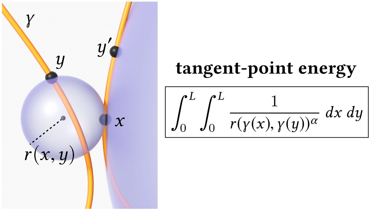
[17/n] The power α just controls how quickly the influence of the curve falls off, yielding somewhat different solutions for different α values. (See the paper for a more detailed discussion of which values can/should be used.)

[18/n] So, this is a pretty simple & slick energy, that doesn't need an ad-hoc definition of "close on the curve" vs. "close in space."

But, some problems:

1. It's expensive to evaluate/optimize, since it considers all pairs of points

2. It's easy to get stuck in local minima

[19/n] To deal with the O(n²) complexity we draw on a bunch of tricks & techniques from n-body literature: Barnes-Hut, hierarchical matrices, and a multi-resolution mesh hierarchy. Have to think a bit to incorporate tangent information—but get massive speedups in the end!

[20/n] The more interesting question is how to navigate the energy landscape. I.e., which direction(s) should we nudge the curve to reduce the energy as fast as possible?

Just doing ordinary (L2) gradient descent takes *forever*, and struggles to slide out of tricky situations.

[21/n] Instead of trying to bludgeon this problem with general-purpose, black-box optimization techniques, we take some queues from functional analysis and differential geometry.

Here we really need to think in terms of *smooth* curves, rather than "all pairs of vertices."

[22/n] The full-blown strategy gets quite technical—so instead I'll consider a much simpler problem:

Minimize the "wiggliness" of an ordinary function on the real line.

I.e., minimize the integral of its squared derivative (Dirichlet energy).

[23/n] A natural idea is to just do gradient descent: find the direction that reduces Dirichlet energy "fastest" and move a bit in that direction.

It's not too hard to show that this strategy is equivalent to heat flow: push the curve down where the 2nd derivative is big.

[24/n] At the beginning, heat flow does a great job of smoothing out small bumps and wrinkles.

But after this initial phase, it takes *forever* to smooth out bigger, lower-frequency oscillations.

[25/n] So, what can you do?

A critical observation is: to talk about the "fastest" descent direction, you must define a notion of size!

I.e., you must pick a norm (or inner product).

And: nobody requires you to use the standard L2 inner product.

[26/n] More precisely:

The *gradient* is the vector whose _inner product_ with any vector X gives the directional derivative along X.

So: a different inner product gives a different (sometimes "better") definition to the gradient.

[27/n] This perspective is one way of explaining Newton's method.

Rather than use the steepest direction in your usual coordinate system—which might zig-zag back and forth across a narrow valley—you switch to a coordinate system where the gradient points straight to the bottom.

[28/n] But Newton's method, famous as it is, is far from perfect:

- The Hessian is expensive to evaluate/invert.
- If it's not convex, you need heuristics to "convexify."
- It works great near minimizers, but not everywhere.

https://twitter.com/keenanisalive/status/1421783338143129603

[29/n] A different starting point are so-called "Sobolev methods."

The ansatz is that gradient descent is a high-order partial differential equation (PDE), which requires *very* small time steps.

So, can we pick an inner product that yields a lower-order gradient descent PDE?

[30/n] Well, let's think again about Dirichlet energy.

The ordinary (L2) gradient flow PDE is 2nd-order in space: heat flow.

But if we use the 2nd-order Laplace operator to define our inner product ("H1") we get a 0th-order gradient equation—which is trivial to integrate!

[31/n] Rather than smoothing out only "little features", this H1 gradient flow smooths out "big features" at the same rate.

So, you can take super-big time steps toward the minimizer (which in this case is just a constant function).

[32/n] We could try going even further, and "remove" even more derivatives—for instance, by using the bi-Laplacian Δ² to precondition the gradient. But this would be a mistake: now gradient flow eliminates low frequencies quickly, but small details stick around for a long time.

[33/n] Here's a plot in a 2D slice of function space. L2 gradient flow quickly eliminates high frequencies, but not low frequencies. H2 kills low but not high frequencies. H1 is just right—at least for Dirichlet energy.

In general: match the inner product to your energy!

[34/n] Sobolev schemes have been used over the years for various problems in simulation and geometry processing.

For instance, the classic algorithm Pinkall & Polthier for minimizing surface area is a Sobolev scheme in disguise—see Brakke 1994 §16.10: facstaff.susqu.edu/brakke/evolver…

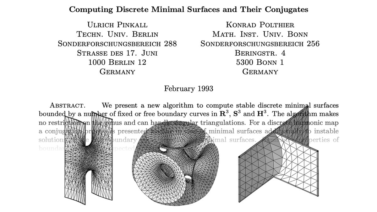
[35/n] Renka & Neuberger 1995 directly considers minimal surfaces and Sobolev gradients:
epubs.siam.org/doi/pdf/10.113…

Since the Laplace operator changes at every point (i.e., for every surface), you can also think of these schemes as gradient descent w.r.t. a Riemannian metric.

[36/n] Many other methods for surface flows adopt this "Sobolev" approach: pick an inner product of appropriate order to take (dramatically) larger steps, e.g.

2007: di.ens.fr/willow/pdfs/07…
2012: cs.utah.edu/docs/techrepor…
2013: cs.cmu.edu/~kmcrane/Proje…
2017: arxiv.org/abs/1703.06469

[37/n] Another nice example is preconditioning for mesh optimization.

For instance, Holst & Chen 2011 suggests H1 preconditioning to accelerate computation of optimal Delaunay triangulations: math.uci.edu/~chenlong/Pape…

(We use this scheme all the time—works great in practice!)

[38/n] In more recent years, Sobolev methods (esp. Laplacian/H1 preconditioning) has become popular for elastic energies for mesh parameterization/deformation:

2016: shaharkov.github.io/projects/Accel…
2017: people.csail.mit.edu/jsolomon/asset…
2018: cs.columbia.edu/~kaufman/BCQN/…

@JustinMSolomon @lipmanya

[39/n] What about tangent-point energy?

Unfortunately we can't just "plug and chug", since the differential of tangent-point energy has *fractional* order.

So, to eliminate all the derivatives, we likewise need to define & invert a *fractional* to inner product.

[40/n] This situation leads down a rabbit hole involving fractional Laplacians and kernel approximations…

A big challenge is that, unlike ordinary (integer-order) operators, the fractional Laplacian is not a local operator—hence we can't use standard computational tools…

[41/n] …But in the end things work out great: a fractional preconditioner works way better than even ordinary "integer" Sobolev preconditioners (H1 and H2) that have been used in past geometry processing methods—and can still be applied efficiently.

[42/n] This efficient fractional preconditioning doesn't merely let us avoid collisions—it enables us to navigate the global energy landscape, and untangle difficult knots way faster than any known method (including tried-and-true packages like KnotPlot).

[43/n] At the risk of re-writing the whole paper on Twitter, I'll just point back to the original source: cs.cmu.edu/~kmcrane/Proje…

Have fun—and hope you're not too repulsed! ;-)