Thread by @alfcnz

This week we went through the second part of my lecture on latent variable 👻 energy 🔋 based models. 🤓

We've warmed up a little the temperature 🌡, moving from the freezing 🥶 zero-temperature free energy Fₒₒ(y) (you see below spinning) to a warmer 🥰 Fᵦ(y).

https://twitter.com/alfcnz/status/1319121960429887488

Be careful with that thermostat! If it's gonna get too hot 🥵 you'll end up killing ☠️ your latents 👻 and end up with averaging them all out, indiscriminately, ending up with plain boring MSE (fig 1.3)! 🤒
From fig 2.1–3, you can see how more z's contribute to Fᵦ(y).

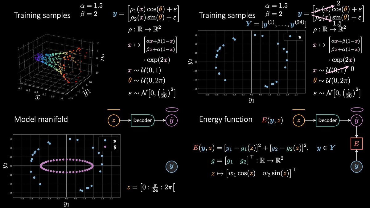
This is nice, 'cos during training (fig 3.3, bottom) *The Force* will be strong with a wider region of your manifold, and no longer with the single Jedi. This in turns will lead to a more even pull and will avoid overfitting (fig 3.3, top). Still, we're fine here because z ∈ ℝ.

Finally, switching to the conditional / self-supervised case, where we introduce an observed x, requires changing 1 line of code! 🤯
Basically, self-sup and un-sup are super close in programming space! 😬
So, learning the horn 📯 was easy peasy! 😎
Made with @matplotlib as usual.

For reference, the (now correct) training data is shown below. Pay attention that ∞ y's (an entire ellipse) are associated to a give x. So, you cannot hope to use a neural net to train on (x, y) pairs. That model would collapse into the segment (0, 0, 0) → (1, 0, 0).

One more note. 🧐
Fig 1.4 shows the *correct* terminology 👍🏻 vs. what is currently commonly used 👎🏻.
Actual softmax → "logsumexp" (scalar).
Its derivative, softargmax → "softmax" (pseudo probability).
This is analogous to max and, its derivative, argmax. But softer. 😀