Thread by @hippopedoid

In a new paper with @JanLause & @CellTypist we argue that the best approach for normalization of UMI counts is *analytic Pearson residuals*, using NB model with an offset term for seq depth. + We analyze related 2019 papers by @satijalab and @rafalab. /1

biorxiv.org/content/10.110…

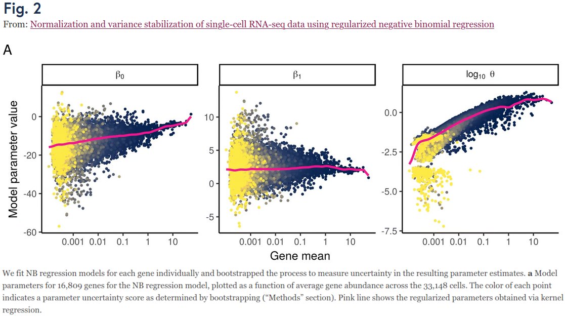
Our project began when we looked at Fig 2 in Hafemeister & Satija 2019 (genomebiology.biomedcentral.com/articles/10.11…) who suggested to use NB regression (w/ smoothed params), and wondered:

1) Why does smoothed β_0 grow linearly?
2) Why is smoothed β_1 ≈ 2.3??
3) Why does smoothed θ grow too??? /2

The original paper does not answer any of that.

Jan figured out that: (1) is trivially true when assuming UMI ~ NB(p_gene * n_cell); (2) simply follows from HS2019 parametrization & the magic constant is 2.3=ln(10); (3) is due to bias in estimation of overdispersion param θ! /3

We argue, based on theory, that NB regression should have sequencing depth (sum of UMI counts per cell) as an _offset_ term and should only have one free parameter, the intercept β_0. In which case it has a simple analytic solution!

And no regularization/smoothing is needed. /4

Moreover, this analytic solution is equivalent to the rank-one GLM-PCA developed in Townes et al. 2019 (genomebiology.biomedcentral.com/articles/10.11…) by @sandakano @stephaniehicks @rafalab. This nicely unifies these two papers that were published back-to-back in @GenomeBiology a year ago. /5

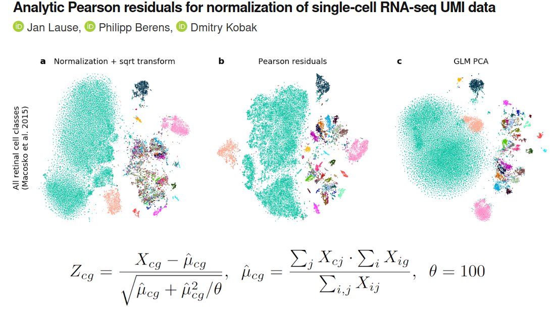
Furthermore, we analyzed several negative control datasets (as @vallens Svensson 2020 did to show that UMI data are not zero-inflated: nature.com/articles/s4158…) and argue that technical overdispersion compared to Poisson is quite low, with technical θ~100 (for all genes). /6

Putting this all together, we get a simple formula for Pearson residuals in closed form. /7

As argued by HS2019 and THAI2019, Pearson residuals can be used for feature selection: simply select genes with the highest variance of Pearson residuals. And for normalization: use Pearson residuals for downstream processing, e.g. t-SNE. /8

Jan analyzed a bunch of different datasets and our conclusion is that (analytic) Pearson residuals tend to work better than normalization + log-transform or sqrt-transform (@flo_compbio), and also better (and much faster!) than the full-blown GLM-PCA. /9

See our preprint (biorxiv.org/content/10.110…) for all the technical details. /10

Christoph and Rahul @satijalab wrote a response arguing that their 'regularized' approach yields a more meaningful gene selection than our 'analytic' approach. Brief reply in the next tweet. But importantly, we all agree that Pearson resid. are cool! /11

https://twitter.com/satijalab/status/1337216550152138752

"Meaningful" PBMC genes listed by H&S as having higher variance in scTransform also have high analytic var (black dots) and would be selected. "Non-meaningful" genes all have much lower var (red dots). The difference is due to θ=100 vs θ≈10, not due to offset/regularization. /12