1/
Get a cup of coffee.
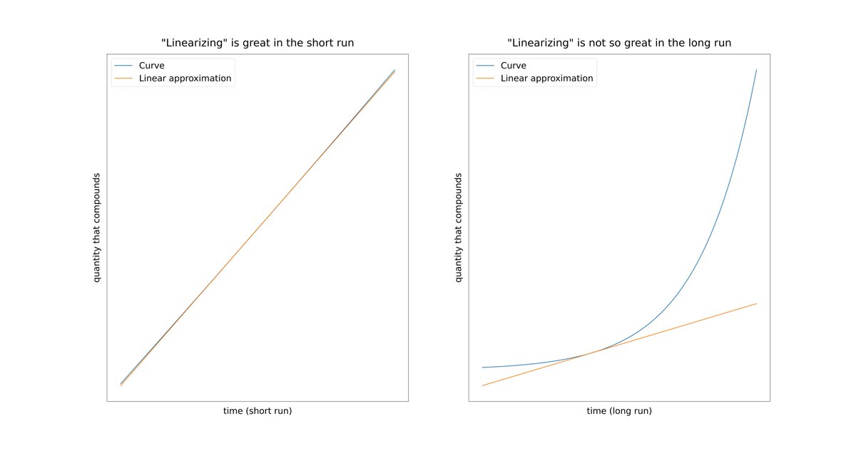
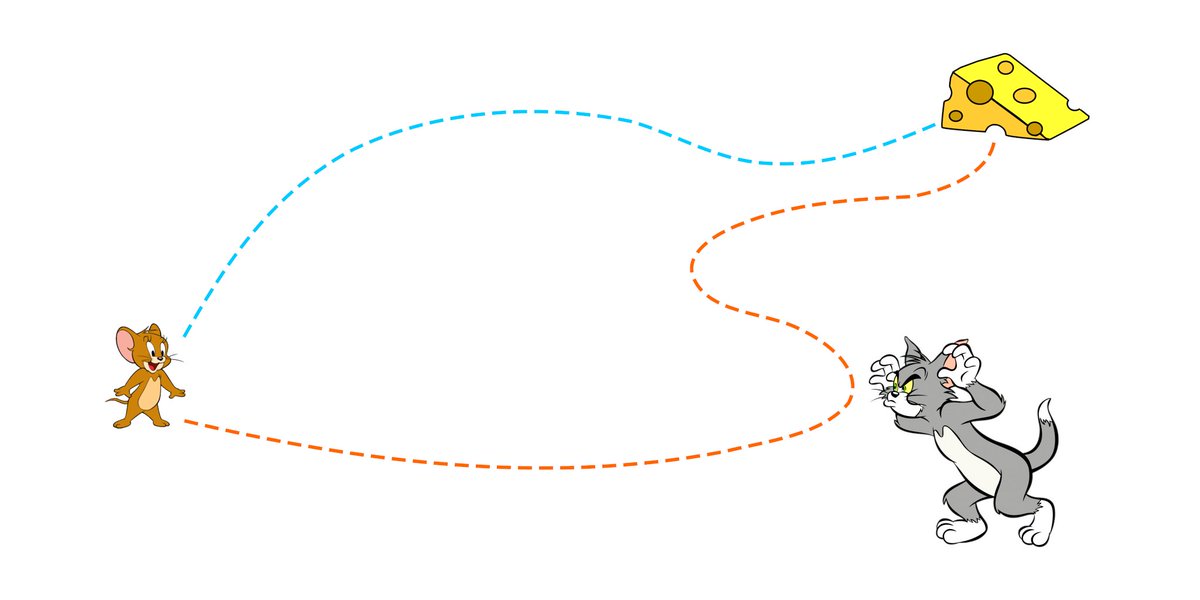
In this thread, I'll walk you through the concept of "path dependence".
This plays such a key role in deciding so many financial outcomes.
And yet, most financial projections completely ignore it.
Get a cup of coffee.
In this thread, I'll walk you through the concept of "path dependence".
This plays such a key role in deciding so many financial outcomes.
And yet, most financial projections completely ignore it.
2/
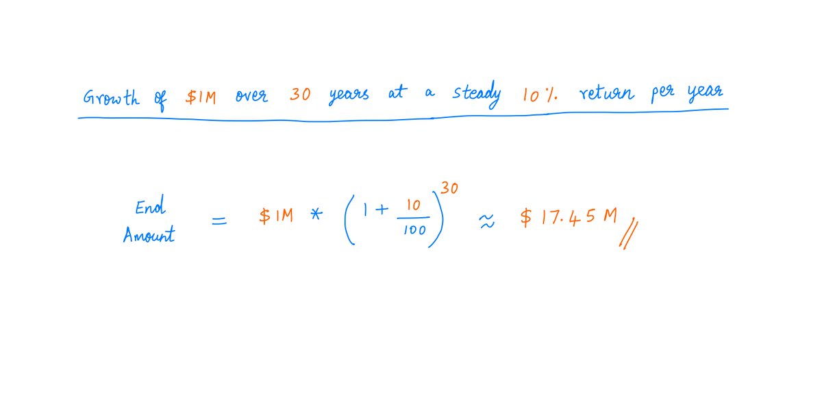
Suppose we have $1M invested in an S&P 500 index fund.
Say, we leave this money untouched for the next 30 years.
If we get a steady 10% per year return over this period, we'll be left with ~$17M.
Not a bad result.
Suppose we have $1M invested in an S&P 500 index fund.
Say, we leave this money untouched for the next 30 years.
If we get a steady 10% per year return over this period, we'll be left with ~$17M.
Not a bad result.
3/
Of course, we probably won't get a *steady* 10% return every year.
Some years, we'll likely make more than 10%. Other years, we may even get a negative return and lose money.
It's all part of the game.
Of course, we probably won't get a *steady* 10% return every year.
Some years, we'll likely make more than 10%. Other years, we may even get a negative return and lose money.
It's all part of the game.
4/
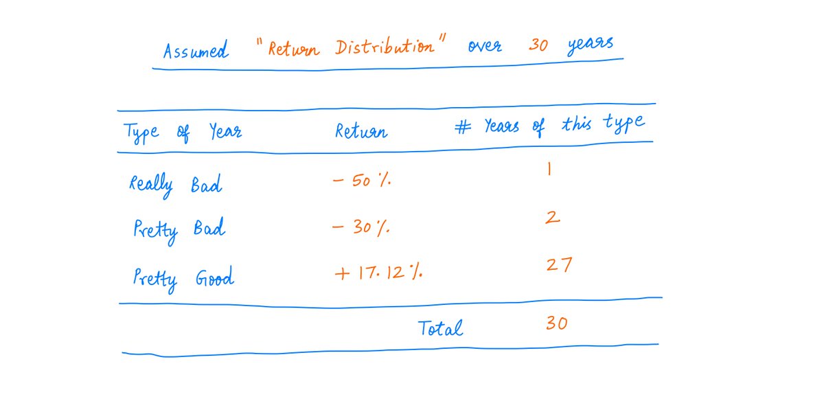
To model this, let's assume that 1 of the next 30 years will be "really bad". We'll lose 50% that year.
And 2 other years will be "pretty bad". Those years, we'll lose 30%.
But to compensate, the other 27 years will be "pretty good". We'll make ~17.12% in each of them.
To model this, let's assume that 1 of the next 30 years will be "really bad". We'll lose 50% that year.
And 2 other years will be "pretty bad". Those years, we'll lose 30%.
But to compensate, the other 27 years will be "pretty good". We'll make ~17.12% in each of them.
5/
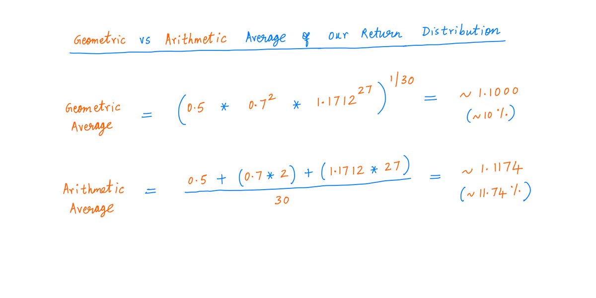
On *average*, our annual return will still be the *same* ~10% over these 30 years.
Note: In such situations, we should calculate averages *geometrically*, not *arithmetically*.
For more:
On *average*, our annual return will still be the *same* ~10% over these 30 years.
Note: In such situations, we should calculate averages *geometrically*, not *arithmetically*.
For more:
https://twitter.com/10kdiver/status/1267150372746833920
6/
Therefore:
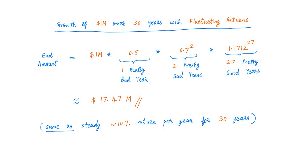
Whether we get a *steady* ~10% per year, or these highly *fluctuating* returns, the end result is the same.
We'll be left with the same ~$17M at the end of 30 years.
Therefore:
Whether we get a *steady* ~10% per year, or these highly *fluctuating* returns, the end result is the same.
We'll be left with the same ~$17M at the end of 30 years.
7/
Also, the *order* doesn't matter.
The "really bad" year, the 2 "pretty bad" years, and the 27 "pretty good" years could be arranged in any order -- and we'll still be left with exactly the same ~$17M after 30 years.
Also, the *order* doesn't matter.
The "really bad" year, the 2 "pretty bad" years, and the 27 "pretty good" years could be arranged in any order -- and we'll still be left with exactly the same ~$17M after 30 years.
8/
This "indifference to order" is a very nice feature.
It means we don't have to worry about predicting which years will be good and which will be bad.
As long as we stay the course and leave the $1M untouched, we'll do pretty well -- if our geometric average is decent.
This "indifference to order" is a very nice feature.
It means we don't have to worry about predicting which years will be good and which will be bad.
As long as we stay the course and leave the $1M untouched, we'll do pretty well -- if our geometric average is decent.
9/
But leaving money *untouched* means neither *adding* to it nor *removing* from it.
Most of us don't invest like that.
As we earn, most of us save and *add* to our investments over time.
And in retirement, most of us *remove* from our investments to meet expenses.
But leaving money *untouched* means neither *adding* to it nor *removing* from it.
Most of us don't invest like that.
As we earn, most of us save and *add* to our investments over time.
And in retirement, most of us *remove* from our investments to meet expenses.
10/
Here's the deal:
When we add and remove money like this, the *order* of up years and down years is no longer irrelevant.
It suddenly becomes *super* important.
Here's the deal:
When we add and remove money like this, the *order* of up years and down years is no longer irrelevant.
It suddenly becomes *super* important.
11/
Let me show you an example.
Say we're just getting started with the "earning, saving, and investing" phase of our journey.
During this phase, we start with $0.
But every year for the next 30 years, we save $100K and add it to our investments.
Let me show you an example.
Say we're just getting started with the "earning, saving, and investing" phase of our journey.
During this phase, we start with $0.
But every year for the next 30 years, we save $100K and add it to our investments.
12/
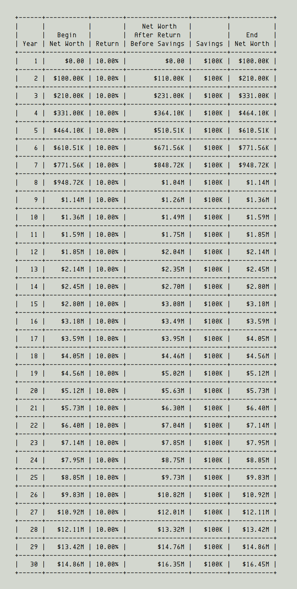
If we get a *steady* 10% return during these 30 years, we'll be left with ~$16M, as this simulation shows:
If we get a *steady* 10% return during these 30 years, we'll be left with ~$16M, as this simulation shows:
13/
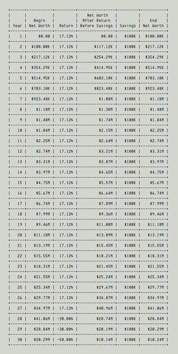
What if we get "front loaded" returns? Good years first, bad years later.
For example, first 27 "pretty good" years. Then, 2 "pretty bad" years. Finally, 1 "really bad" year.
Now, we'll only be left with $10M. Not ~$16M.
See? The *order* makes a huge difference.
What if we get "front loaded" returns? Good years first, bad years later.
For example, first 27 "pretty good" years. Then, 2 "pretty bad" years. Finally, 1 "really bad" year.
Now, we'll only be left with $10M. Not ~$16M.
See? The *order* makes a huge difference.
14/
What if it's the reverse -- "back loaded" returns? Bad years first, good years later.
Now, it turns out, we'll end up with almost 6 times as much money -- ~$57M!
What if it's the reverse -- "back loaded" returns? Bad years first, good years later.
Now, it turns out, we'll end up with almost 6 times as much money -- ~$57M!
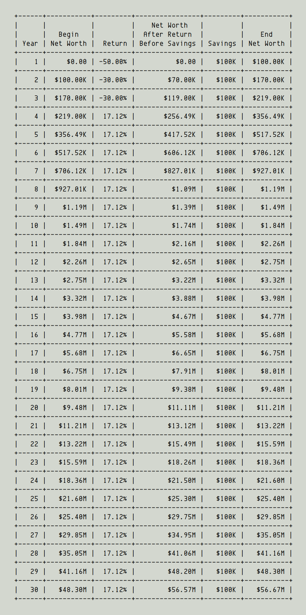
15/
During 30 years of earning, saving, and investing, a few bad years are inevitable.
It's far better to be hit by these years *early*, rather than *late*.
Why? Because, early on, we only have small amounts of capital. At this stage, a bad year or two can't do big damage.
During 30 years of earning, saving, and investing, a few bad years are inevitable.
It's far better to be hit by these years *early*, rather than *late*.
Why? Because, early on, we only have small amounts of capital. At this stage, a bad year or two can't do big damage.
16/
So, to be hit by a big crash just as we're getting started may *seem* like an unlucky thing.
But it may in fact be a blessing in disguise.
The important thing is to stay calm and continue to invest intelligently.
To *not* get discouraged and abandon the pursuit.
So, to be hit by a big crash just as we're getting started may *seem* like an unlucky thing.
But it may in fact be a blessing in disguise.
The important thing is to stay calm and continue to invest intelligently.
To *not* get discouraged and abandon the pursuit.
17/
"Path dependence" is basically this idea -- that "front loaded" vs "back loaded" returns can result in starkly different financial outcomes.
In our example, the difference was a net worth of ~$10M vs ~$57M.
"Path dependence" is basically this idea -- that "front loaded" vs "back loaded" returns can result in starkly different financial outcomes.
In our example, the difference was a net worth of ~$10M vs ~$57M.
18/
Unfortunately, most financial projections I've seen don't consider this super important effect.
They blithely assume a *steady* 7% or 10% return and completely ignore path dependence. This can lead us to make dangerous financial decisions.
Unfortunately, most financial projections I've seen don't consider this super important effect.
They blithely assume a *steady* 7% or 10% return and completely ignore path dependence. This can lead us to make dangerous financial decisions.
19/
Therefore, when we make financial projections, it's a good idea to simulate different scenarios to work out the impact of path dependence.
We can hope for good paths (eg, steady or back loaded returns).
But we must also be prepared for bad paths (eg, front loaded returns).
Therefore, when we make financial projections, it's a good idea to simulate different scenarios to work out the impact of path dependence.
We can hope for good paths (eg, steady or back loaded returns).
But we must also be prepared for bad paths (eg, front loaded returns).
20/
As you may have guessed, what's a *good* path when we're *adding* money is a *bad* path when we're *removing* money.
During retirement, for example, we should hope for *front loaded* returns. Bad years early on can wipe our retirement portfolio and make us run out of money.
As you may have guessed, what's a *good* path when we're *adding* money is a *bad* path when we're *removing* money.
During retirement, for example, we should hope for *front loaded* returns. Bad years early on can wipe our retirement portfolio and make us run out of money.
21/
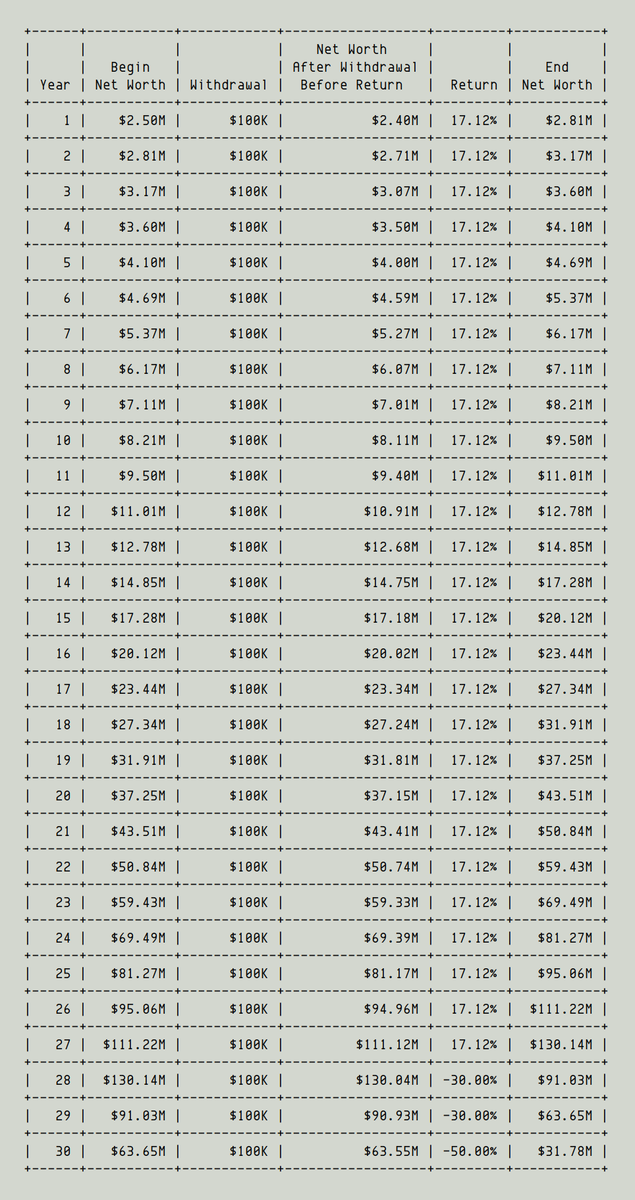
For example, suppose we want to withdraw $100K per year from our portfolio to meet our expenses during retirement.
Following the "4% Rule", let's say we start with a $2.5M portfolio.
We'll probably be OK if we get front loaded returns:
For example, suppose we want to withdraw $100K per year from our portfolio to meet our expenses during retirement.
Following the "4% Rule", let's say we start with a $2.5M portfolio.
We'll probably be OK if we get front loaded returns:
22/
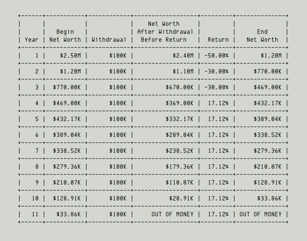
But if we get back loaded returns (bad years early on during retirement), there's a real danger of running out of money -- as the simulation below shows.
For more on retirement planning, the 4% Rule, and such:
But if we get back loaded returns (bad years early on during retirement), there's a real danger of running out of money -- as the simulation below shows.
For more on retirement planning, the 4% Rule, and such:
https://twitter.com/10kdiver/status/1287043526153273344
23/
Path dependence also plays a big role when companies do share buybacks.
For example, suppose we own stock in a company that regularly buys back a lot of shares.
Say we buy the stock at time t_buy, and sell it at time t_sell.
Path dependence also plays a big role when companies do share buybacks.
For example, suppose we own stock in a company that regularly buys back a lot of shares.
Say we buy the stock at time t_buy, and sell it at time t_sell.
24/
Of course, at t_sell, we should hope for the stock to trade at a high multiple of earnings.
But *between* t_buy and t_sell, we'd be better off if the stock price *languished* -- allowing the company to buy back more shares on the cheap. Another example of path dependence.
Of course, at t_sell, we should hope for the stock to trade at a high multiple of earnings.
But *between* t_buy and t_sell, we'd be better off if the stock price *languished* -- allowing the company to buy back more shares on the cheap. Another example of path dependence.
25/
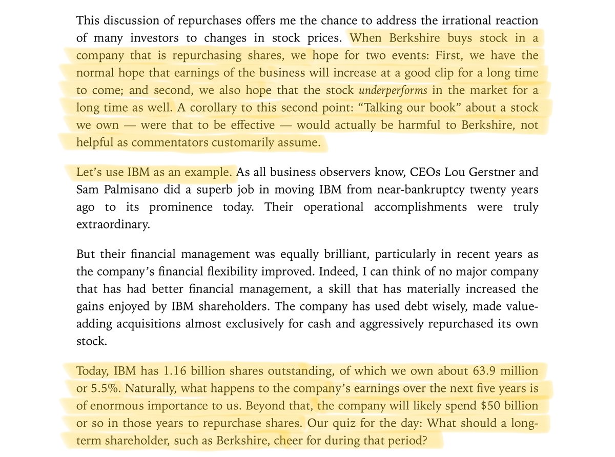
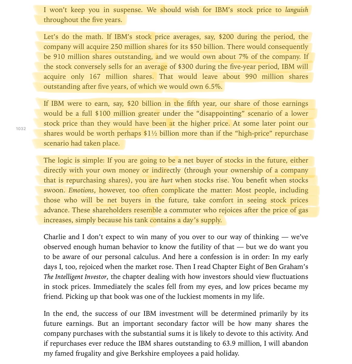
As Buffett explained in his 2011 letter:
(He used IBM as an example to illustrate this, which was perhaps unfortunate as the investment didn't work out for Berkshire. But the principle still holds.)

As Buffett explained in his 2011 letter:
(He used IBM as an example to illustrate this, which was perhaps unfortunate as the investment didn't work out for Berkshire. But the principle still holds.)
26/
An extreme example of path dependence can occur when investors take too much risk with leverage, margin loans, shorting stocks, etc.
Even if they're right about the underlying business, the *path* followed by its stock price can wipe them out.
An extreme example of path dependence can occur when investors take too much risk with leverage, margin loans, shorting stocks, etc.
Even if they're right about the underlying business, the *path* followed by its stock price can wipe them out.
27/
The title of a chapter in @Gautam__Baid's book, The Joys of Compounding, says it all:
To finish first, you must first finish.
And if we take reckless risks, path dependence can get us thrown out of the game.
The title of a chapter in @Gautam__Baid's book, The Joys of Compounding, says it all:
To finish first, you must first finish.
And if we take reckless risks, path dependence can get us thrown out of the game.
28/
If you're still with me, kudos!
Paraphrasing Robert Frost, you took the path less traveled -- all the way to the end of this thread.
And that, to me, makes all the difference.
Thank you very much. Stay safe. Enjoy your weekend!
/End
If you're still with me, kudos!
Paraphrasing Robert Frost, you took the path less traveled -- all the way to the end of this thread.
And that, to me, makes all the difference.
Thank you very much. Stay safe. Enjoy your weekend!
/End
• • •
Missing some Tweet in this thread? You can try to
force a refresh

