Thread by @daansan_ml

Don't forecast future values in Time Series using the traditional way!! ⛔

Discover the Rolling forecasting! 🤯

#python #machinelearning #ml #ai #datascience

Yesterday we discussed the first way of forecasting with your Time Series model:
1️⃣ The traditional way or multi-step forecast

Today is time for the second (and better) way:

2️⃣ Rolling forecast

2️⃣ Rolling forecast

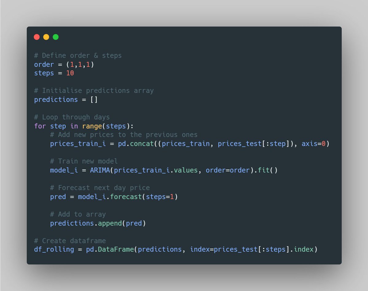
As mentioned yesterday, this consists of training the model every day, with all the available data until the present day.

Then we forecast for tomorrow.

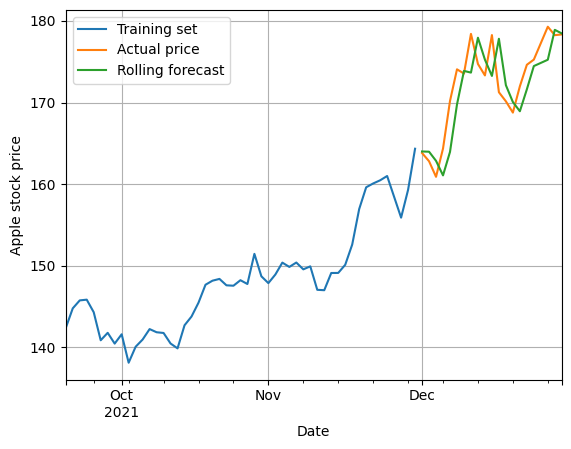
Let's continue with yesterday's example.

The data we used was the Apple stock price.

We assumed that today was 30/11/2021.

We split the data in two:
- Training: prices until "today"
- Testing: prices from "today"

- Training set to train the model.

- Testing set to evaluate the results, as this is the Actual price to match.

This will consider all the available data, which will significantly improve the predictions! 🤯

NOTE: this data or model are not the best ones, so this model seems to kind of replicate the previous price. This was not the purpose of this thread, so we will not focus on that.

▶️ TL;DR

The rolling forecasting method is a much better way of evaluating your Time Series model.

The traditional method performs poorly as it does not consider all the available data.

Check yesterday's thread about the Traditional forecasting method 👇

https://twitter.com/daansan_ml/status/1611020333993328640

Please 🔁Retweet the FIRST tweet if you found it useful!

🔔 Follow me @daansan_ml if you are interested in:

🐍 #Python
📊 #DataScience
📈 #TimeSeries
🤖 #MachineLearning

Thanks! 😉