Thread by @alfcnz

#AcademicChatter

Coming from engineering, I'm a former @MATLAB user, moved to @TorchML and @LuaLang, then to @PyTorch and @ThePSF @RealPython, and now I'm exploring @WolframResearch @stephen_wolfram.
For learning, one would prefer knowledge packed frameworks and documentation.

In that regard, @MATLAB and @WolframResearch are ridiculously compelling. The user manuals are just amazing, with everything organised and available at your disposal. Moreover, the language syntax is logical, much closer to math, and aligned to your mental flow.

In Mathematica I can write y = 2x (implicit multiplication), x = 6, and y will be now equal 12. y is a variable.
Or I can create a function of x with y[x_] := 2x (notice that x_ means I don't evaluate y right now). Later, I can execute y[x] and get 12, as above.

If I write "3d graph x+y+z=0", this comes out. If I'd need to do the same, say, in @matplotlib, I should write 10 to 20 lines of code. My question is whether I'm using the wrong tool for what I'm trying to do.

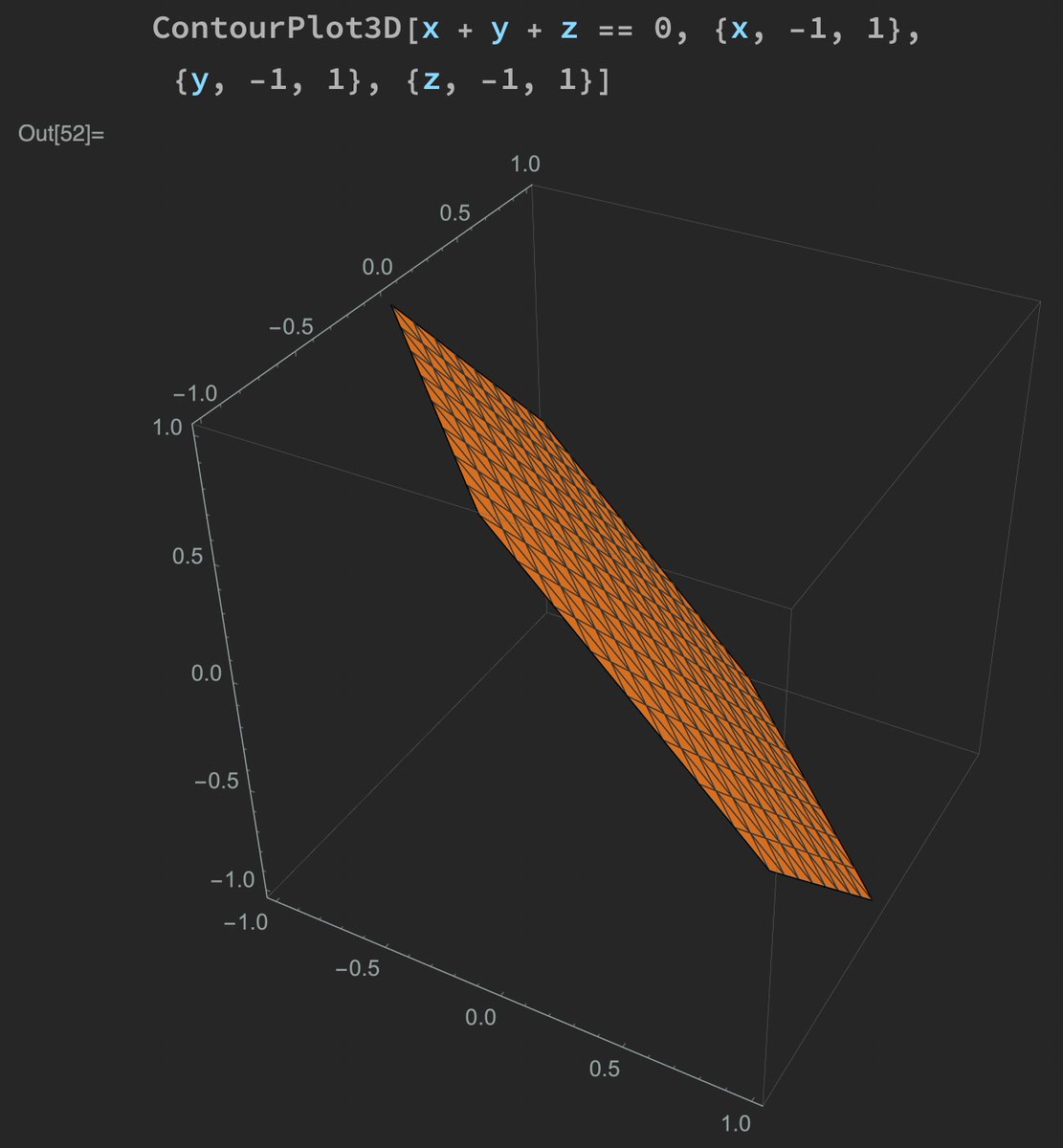
Now I understand that one *can* use Python / Numpy / Matplotlib to do math, but this becomes very expensive for the user. Writing the English one-liner vs. correctly putting together the 20 lines of commands is quite a substantial difference.

Knowing *what* package to import and *how* to use it is quite daunting. Yeah, with Python you can do *everything*, but this doesn't mean you should. Right?

Math colleagues, what is your take? What tools do you use and for what? How about education vs. research?

Ping @CentrlPotential, @bencbartlett, @matthen2, @3blue1brown, @InertialObservr, @rickyreusser, @KangarooPhysics, @AndrewM_Webb, @jezzamonn, @jcponcemath.