1/🧵✨Occam's razor is a principle that states that the simplest explanation is often the best one. But did you know that it can also be applied to statistics? Let's dive into how Occam's razor helps us make better decisions in data analysis. #OccamsRazor#Statistics#DataScience
2/ 📏 Occam's razor is based on the idea of "parsimony" - the preference for simpler solutions. In statistics, this means choosing models that are less complex but still accurate in predicting outcomes. #Simplicity#DataScience
3/ 📊 Overfitting is a common problem in statistics, where a model becomes too complex and captures noise rather than the underlying trend. Occam's razor helps us avoid overfitting by prioritizing simpler models with fewer parameters. #Overfitting#ModelSelection#DataScience
4/ 🔍 A popular application of Occam's razor in statistics is model selection using Akaike Information Criterion (AIC) and Bayesian Information Criterion (BIC). Both criteria add a penalty for the complexity of the model, favoring simpler models. #DataScience#ModelSelection
5/ 🧪 In experimental design, Occam's razor can guide us to focus on fewer variables and interactions, making it easier to detect true effects and reduce the risk of false positives. #ExperimentalDesign#Science#DataScience
6/ 📚 Occam's razor reminds us that complexity isn't always better. In statistics, embracing simplicity can lead to more robust, interpretable, and generalizable results. Keep it simple, and let the data speak for itself! #DataDriven#KeepItSimple#DataScience
• • •
Missing some Tweet in this thread? You can try to
force a refresh
[1/9] 🎲 Let's talk about the difference between probability and likelihood in #statistics. These two terms are often confused, but understanding their distinction is key for making sense of data analysis! #Rstats#DataScience
[2/9]💡Probability is a measure of how likely a specific outcome is in a random process. It quantifies the degree of certainty we have about the occurrence of an event. It ranges from 0 (impossible) to 1 (certain). The sum of probabilities for all possible outcomes is always 1.
[3/9] 📊 Likelihood, on the other hand, is a measure of how probable a particular set of observed data is, given a specific set of parameters for a statistical model. Likelihood is not a probability, but it shares the same mathematical properties (i.e., it's always non-negative).
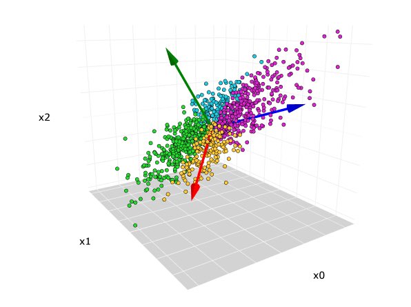
1/🧵🔍 Making sense of Principal Component Analysis (PCA), Eigenvectors & Eigenvalues: A simple guide to understanding PCA and its implementation in R! Follow this thread to learn more! #RStats#DataScience#PCA
2/📚PCA is a dimensionality reduction technique that helps us to find patterns in high-dimensional data by projecting it onto a lower-dimensional space. It's often used for data visualization, noise filtering, & finding variables that explain the most variance. #DataScience
3/🎯 The goal of PCA is to identify linear combinations of original variables (principal components) that capture the maximum variance in the data, with each principal component being orthogonal to the others. #RStats#DataScience
[1/10] 🚀 Advanced R Debugging: Debugging & error handling are essential skills for every R programmer. In this thread, we'll explore powerful tools & techniques like traceback(), browser(), & conditional breakpoints to make debugging in R a breeze. #rstats#datascience
[2/10] 📝 traceback(): When your code throws an error, use traceback() to get a detailed call stack. This function helps you identify the exact location of the error in your code, making it easier to pinpoint the issue. #rstats#debugging#datascience
[3/10] 🔍 browser(): With browser(), you can pause the execution of your code & step through it one line at a time. This interactive debugging tool allows you to inspect the values of variables and expressions, which can be a game-changer when diagnosing complex issues. #rstats
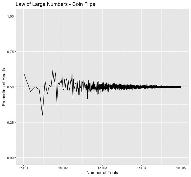
Hello #Rstats community! Today, we're going to explore the Law of Large Numbers (LLN), a fundamental concept in probability theory, and how to demonstrate it using R. Get ready for some code! 🚀
LLN states that as the number of trials (n) in a random experiment increases, the average of the outcomes converges to the expected value. In other words, the more we repeat an experiment, the closer we get to the true probability.
Imagine flipping a fair coin. The probability of getting heads (H) is 0.5. As we increase the number of flips, the proportion of H should approach 0.5. Let's see this in action with R!
1/🧵 Welcome to this thread on the Central Limit Theorem (CLT), a key concept in statistics! We'll cover what the CLT is, why it's essential, and how to demonstrate it using R. Grab a cup of coffee and let's dive in! ☕️ #statistics#datascience#rstats
2/📚 The Central Limit Theorem states that the distribution of sample means approaches a normal distribution as the sample size (n) increases, given that the population has a finite mean and variance. It's a cornerstone of inferential statistics! #CLT#DataScience#RStats
3/🔑 Why is the CLT important? It allows us to make inferences about population parameters using sample data. Since many statistical tests assume normality, CLT gives us the foundation to apply those tests even when the underlying population is not normally distributed. #RStats
[1/11] 🚀 Level Up Your R Machine Learning Skills with These Lesser-Known #RPackages! In this thread, we'll explore 10 hidden gems that can help you optimize your #MachineLearning workflows in R. Let's dive in! 🌊 #rstats#datascience