The fourth episode (of five) of the energy 🔋 saga is out! 🤩
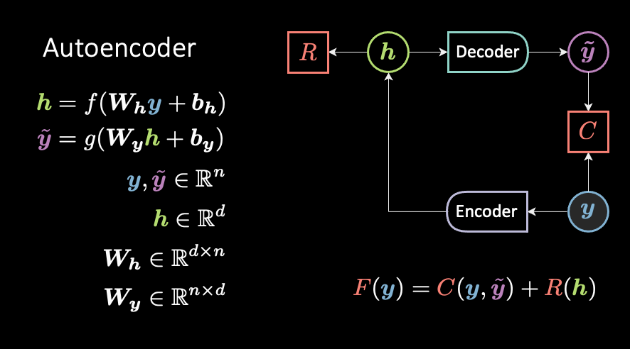
From LV EBM to target prop(agation) to vanilla autoencoder, and then denoising, contractive, and variational autoencoders. Finally, we learn about the VAE's bubble-of-bubbles interpretation.
Edit: updating a thumbnail and adding one more.
In this episode I *really* changed the content wrt last year. Being exposed to EBMs for several semesters now made me realise how all these architectures (and more to come) are connected to each other.
In the companion lecture (which will soon come online), @ylecun goes over a more powerful interpretation of VAE, which I still struggle to understand. As you can imagine, another tweak to my deck will occur when I'll actually get it. (Yeah, I'm slow, yet persistent.)
In this lesson you'll also learn the step-by-step solution to ⁂ Quiz #5 ⁂. A powerful tool to add to your portfolio of useful architectures. More precisely, if it's hard to get it in one go, break it down in smaller chunks.
Moreover, you will also find the solution to ⁂ Quiz #3 ⁂. In case you haven't seen these before, I highly recommend trying them out *before* watching this episode. Struggling a little and engaging in critical thinking will be highly beneficial for you.
Speaking about the transformer architecture, one may incorrectly talk about an encoder-decoder architecture. But this is *clearly* not the case.
The transformer architecture is an example of encoder-predictor-decoder architecture, or a conditional language-model.
The classical definition of an encoder-decoder architecture is the autoencoder (AE). The (blue / cold / low-energy) target y is auto-encoded. (The AE slides are coming out later today.)
Now, the main difference between an AE and a language-model (LM) is that the input is delayed by one unit. This means that a predictor is necessary to estimate the hidden representation of a *future* symbol.
It's similar to a denoising AE, where there is a temporal corruption.
In that regard, @MATLAB and @WolframResearch are ridiculously compelling. The user manuals are just amazing, with everything organised and available at your disposal. Moreover, the language syntax is logical, much closer to math, and aligned to your mental flow.
In Mathematica I can write y = 2x (implicit multiplication), x = 6, and y will be now equal 12. y is a variable.
Or I can create a function of x with y[x_] := 2x (notice that x_ means I don't evaluate y right now). Later, I can execute y[x] and get 12, as above.
This week we went through the second part of my lecture on latent variable 👻 energy 🔋 based models. 🤓
We've warmed up a little the temperature 🌡, moving from the freezing 🥶 zero-temperature free energy Fₒₒ(y) (you see below spinning) to a warmer 🥰 Fᵦ(y).
Be careful with that thermostat! If it's gonna get too hot 🥵 you'll end up killing ☠️ your latents 👻 and end up with averaging them all out, indiscriminately, ending up with plain boring MSE (fig 1.3)! 🤒
From fig 2.1–3, you can see how more z's contribute to Fᵦ(y).
This is nice, 'cos during training (fig 3.3, bottom) *The Force* will be strong with a wider region of your manifold, and no longer with the single Jedi. This in turns will lead to a more even pull and will avoid overfitting (fig 3.3, top). Still, we're fine here because z ∈ ℝ.
This week we've learnt how to perform inference with a latent variable 👻 energy 🔋 based model. 🤓
These models are very convenient when we cannot use a standard feed-forward net that maps vector to vector, and allow us to learn one-to-many and many-to-one relationships.
Take the example of the horn 📯 (this time I drew it correctly, i.e. points do not lie on a grid 𐄳). Given an x there are multiple correct y's, actually, there is a whole ellipse (∞ nb of points) that's associated with it!
Or, forget the x, even considering y alone…
there are (often) two values of y₂ per a given y₁! Use MSE and you'll get a point in the middle… which is WRONG.
What's a “latent variable” you may ask now.
Well, it's a ghost 👻 variable. It was indeed used to generate the data (θ) but we don't have access to (z).
🥳 NEW LECTURE 🥳
Graph Convolutional Networks… from attention!
In attention 𝒂 is computed with a [soft]argmax over scores. In GCNs 𝒂 is simply given, and it's called "adjacency vector".
Slides: github.com/Atcold/pytorch…
Notebook: github.com/Atcold/pytorch…
Summary of today's class.
Slide 1: *shows title*.
Slide 2: *recalls self-attention*.
Slide 3: *shows 𝒂, points out it's given*.
The end.
Literally!
I've spent the last week reading everything about these GCNs and… LOL, they quickly found a spot in my mind, next to attention!
The key concept here is the *sparsity* (constraints) of the graph.
In self-attention, every element in the set looks at each and every other element.
If a sparse graph is given, we limit each element (node / vertex) to look only at a few other elements (nodes / vertices).
🥳 NEW LECTURE 🥳
“Set to set” and “set to vector” mappings using self/cross hard/soft attention. We combined a (two) attention module(s) with a (two) k=1 1D convolution to get a transformer encoder (decoder).
Slides: github.com/Atcold/pytorch…
Notebook: github.com/Atcold/pytorch…
This week's slides were quite dense, but we've been building up momentum since the beginning of class, 3 months ago.
We recalled concepts from:
• Linear Algebra (Ax as lin. comb. of A's columns weighted by x's components, or scalar products or A's rows against x)
• Recurrent Nets (stacking x[t] with h[t–1] and concatenating W_x and W_h)
• Autoencoders (encoder-decoder architecture)
• k=1 1D convolutions (that does not assume correlation between neighbouring features and act as a dim. adapter)
and put in practice with @PyTorch.