Learn all about self-supervised learning for vision with @imisra_!
In this lecture, Ishan covers pretext invariant rep learning (PIRL), swapping assign. of views (SwAV), audiovisual discrimination (AVID + CMA), and Barlow Twins redundancy reduction.

In this lecture, Ishan covers pretext invariant rep learning (PIRL), swapping assign. of views (SwAV), audiovisual discrimination (AVID + CMA), and Barlow Twins redundancy reduction.

Here you can find the @MLStreetTalk's interview, where these topics are discussed in a conversational format.
https://twitter.com/MLStreetTalk/status/1406884357185363974
Here, instead, you can read an accessible blog post about these topics, authored by @imisra_ and @ylecun.
https://twitter.com/ylecun/status/1367516830542270467
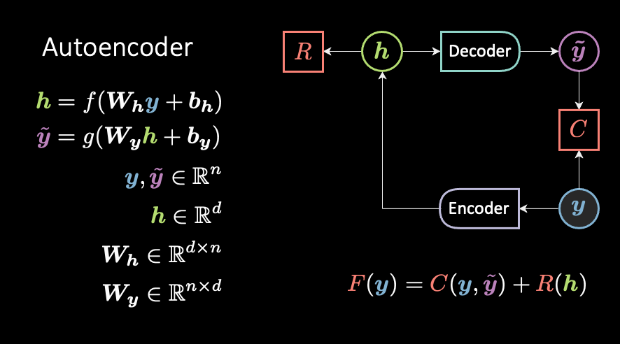
We can organise different classes of joint-embeddings methods in 4 main categories.
• Contrastive (explicit use of negative samples)
• Clustering
• Distillation
• Redundancy reduction
• Contrastive (explicit use of negative samples)
• Clustering
• Distillation
• Redundancy reduction

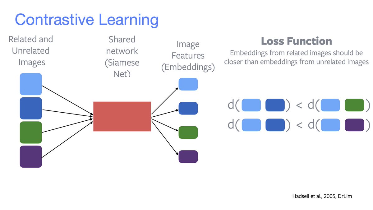
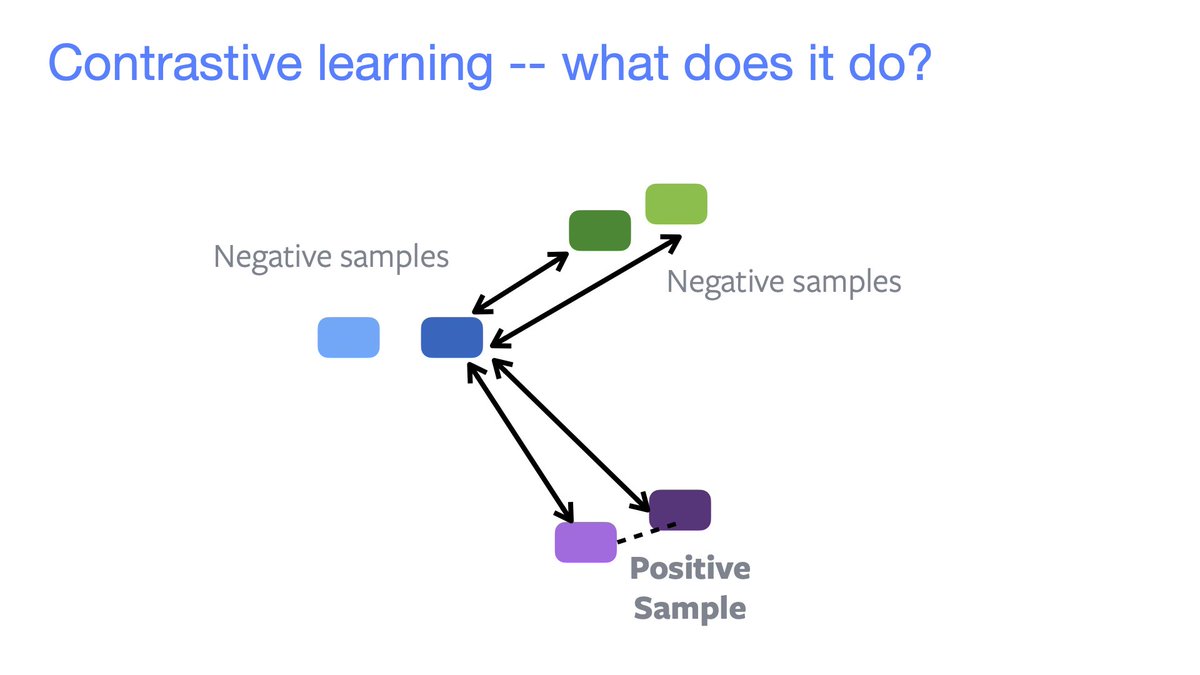
«Contrastive»
Related embeddings (same colour) should be closer than unrelated embeddings (different colour).
Good negatives samples are *very* important. E.g.
• SimCLR has a *very large* batch size;
• Wu2018 uses an offline memory bank;
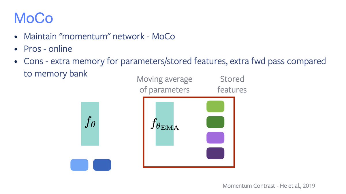
• MoCo uses an “online mem bank”.
Related embeddings (same colour) should be closer than unrelated embeddings (different colour).
Good negatives samples are *very* important. E.g.
• SimCLR has a *very large* batch size;
• Wu2018 uses an offline memory bank;
• MoCo uses an “online mem bank”.


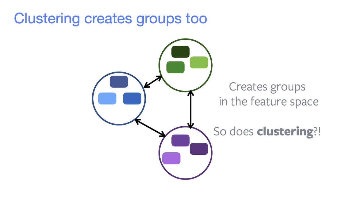
«Clustering»
Contrastive learning ⇒ grouping in feature space.
We may simply want to assign an embedding to a given cluster. Examples are:
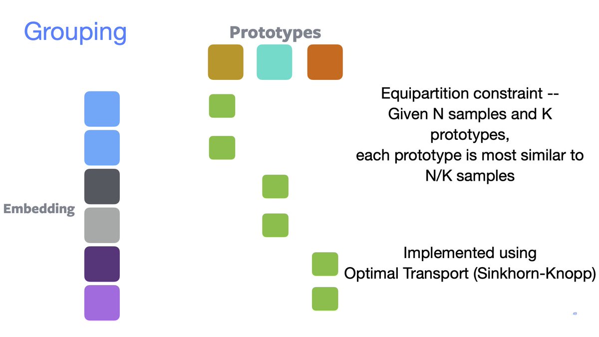
• SwAV performs online clustering using optimal transport;
• DeepClustering;
• SeLA.
Contrastive learning ⇒ grouping in feature space.
We may simply want to assign an embedding to a given cluster. Examples are:
• SwAV performs online clustering using optimal transport;
• DeepClustering;
• SeLA.

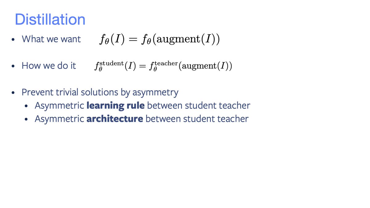
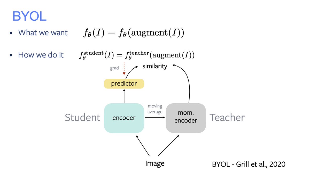
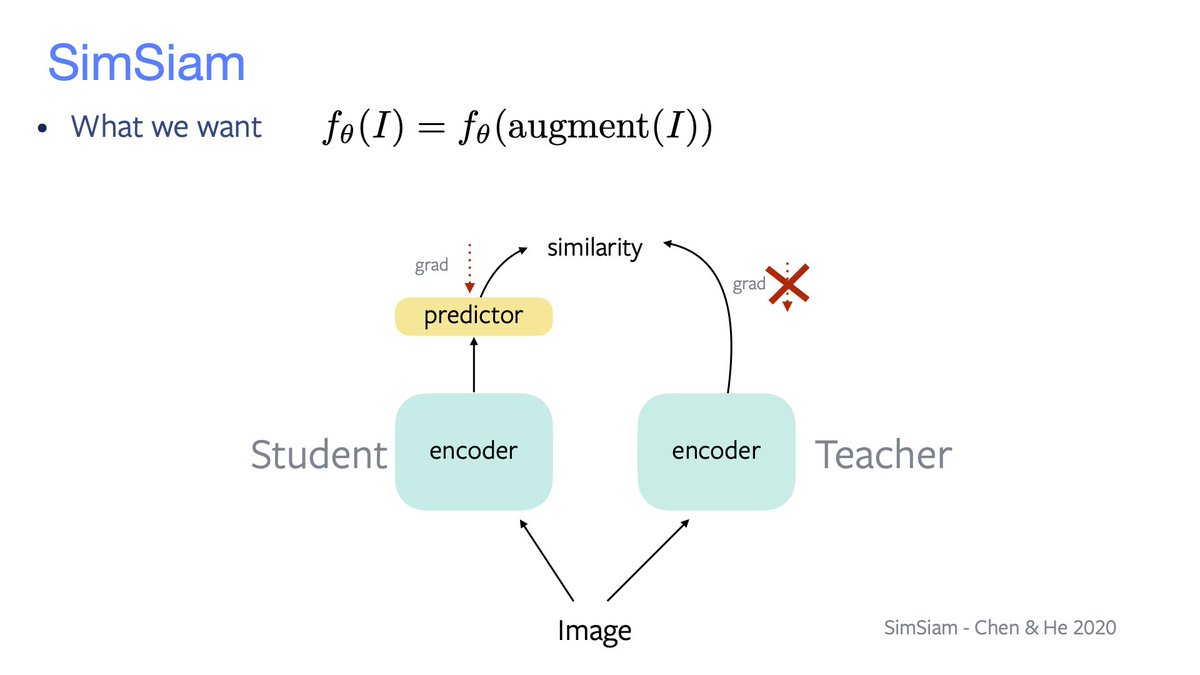
«Distillation»
Similarity maximisation through a student-teacher distillation process. Trivial solution avoided by using asymmetries: learning rule and net's architecture.
• BYOL's student has a predictor on top, the teacher is a slow student;
• SimSiam shares weights.
Similarity maximisation through a student-teacher distillation process. Trivial solution avoided by using asymmetries: learning rule and net's architecture.
• BYOL's student has a predictor on top, the teacher is a slow student;
• SimSiam shares weights.
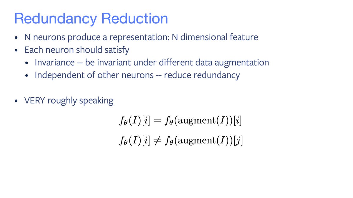
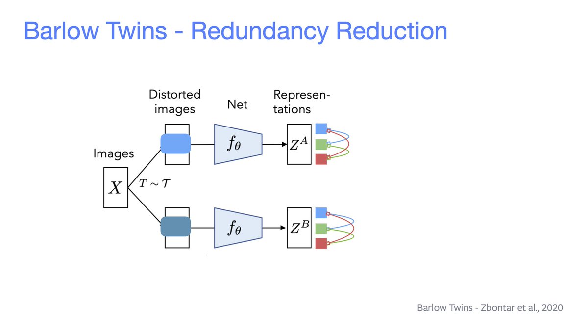
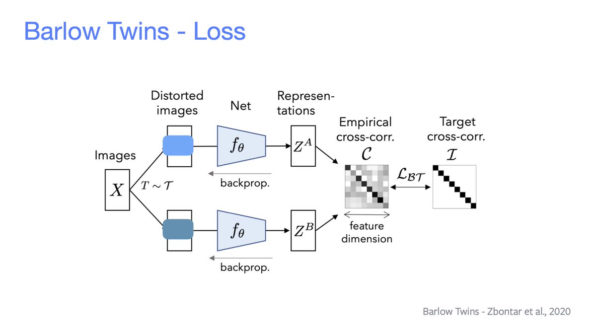
«Redundancy reduction»
Each neuron's representation should be invariant under input data augmentation and independent from other neurons. Everything's done *without* looking at negative examples!
E.g. Barlow Twins makes the covariance close to an identity matrix.
Each neuron's representation should be invariant under input data augmentation and independent from other neurons. Everything's done *without* looking at negative examples!
E.g. Barlow Twins makes the covariance close to an identity matrix.

• • •
Missing some Tweet in this thread? You can try to
force a refresh