Thread by @BenYAndrew

I took a crack at reworking @statsepi’s RCT adjustment post (bit.ly/2Pd1JkH) w/ added simulation & visualization. To pique interest, here is a redacted version of the final image. Stick around for a walkthrough of how to get there & what it means. #epitwitter #rstats 1/n

Let's say we are studying the effect of a treatment on a continuous outcome (Y). In this field of study, 20 continuous patient variables are commonly reported (i.e., are found in the typical table 1). 2/n

Next, let's say that 10 of these variables are causally unrelated to Y (and thus are non-predictors of Y; call these N) and 10 have true causal effects on Y (and thus are predictors of Y; call these C). 3/n

Let's also say that 3 of the causal variables (C1-3) are stronger predictors of Y compared to the others (C4-10). First, let's simulate a large population (5 million) in which each patient has a random vector of the 20 variables w/ an outcome Y (w/o treatment) based on C1-10. 4/n

We can now visualize the population (or a subset of it to reduce over-plotting) to prove to ourselves that we have 10 true non-predictors (N) and 10 predictors (C) in relation to the outcome (Y) under no treatment. Notice that C1-3 are in fact stronger predictors than C4-10. 5/n

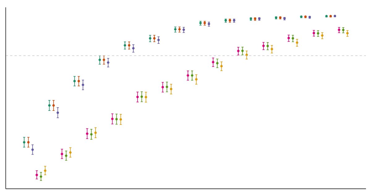
Next, without incorporating a treatment effect, let’s randomly sample from our population (10,000 samples, each w/ n = 500). We’ll randomly divide each sample in half and test for differences in our 20 variables between groups. We can explore these data in several ways. 6/n

For the remainder of this thread, I'll use the term ”imbalanced" or "imbalance" to refer to situations when the P-value for comparison across groups is < 0.05. 7/n

Here we plot the dist. of P-values for comparisons of variables across groups. We see the expected uniform dist. of P-values under the null, with 5% < 0.05. As expected, a variable’s causal relationship to Y does not change the likelihood of imbalance b/w randomized groups. 8/n

Next, we can look at the distribution for the # of imbalanced variables across samples. Given that groups are randomly split, these plots are appropriately reflective of the Binomial distribution with B(n=20, p=0.05) for the left and B(n=10, p=0.05) for the middle & right. 9/n

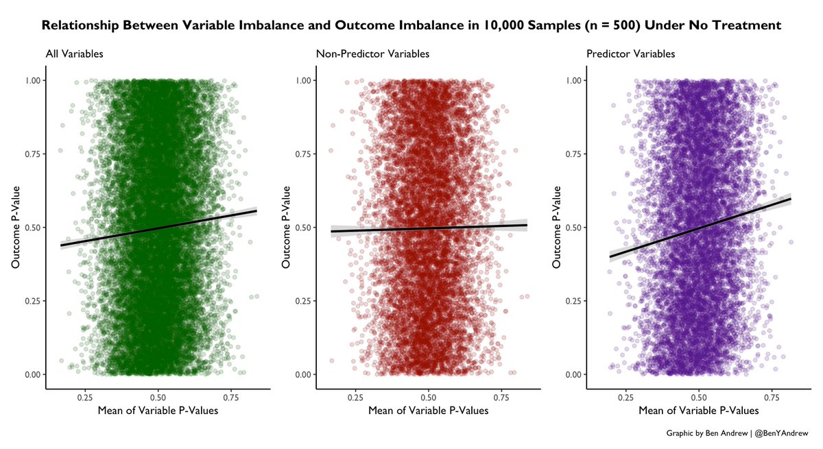
What about the relationship b/w # of imbalanced variables and the likelihood of imbalance in the outcome? Here we see there is no association for # of imbalanced non-predictors, but there is a "dose-response" association present for the # of imbalanced predictor variables. 10/n

Despite randomization, more imbalance in predictor variables = more likely imbalance in Y. This can be visualized in another way: for each sample, the relationship b/w the mean P-val for all vars and the P-val for Y. Again, more imbalance in predictors = more imbalance in Y. 11/n

So far we've seen:

(1) The causal relationship b/w a variable and Y has no impact on its likelihood for being imbalanced b/w randomized groups.

(2) A higher burden of chance imbalances in predictor variables does impart a higher likelihood of imbalance in Y.

12/n

Now let's get back to the goal: estimating a treatment effect.

From this point on, each time we sample from the population we'll add a treatment effect of 0.25 to half of the sample and try to recover this value in our models.

13/n

For the next 2 plots, we'll take 10,000 samples from the pop., randomize and apply 6 models w/ diff. adjustment strategies:

1. No adjustment
2. All imbalanced variables
3. Imbalanced predictors only
4. All variables
5. Strong predictors (C1-3)
6. All predictors (C1-10)

14/n

In this plot, sample size = 300. Adj. strategy is listed to the right.

Left: Density plots for the treatment estimate (dashed line = actual value)

Middle: Density plots for the SE of the treatment estimate

Right: Relative dist. of P-values for the treatment estimate

15/n

This plot tells us 4 major things:

1. All strategies appear to be unbiased (all est. centered at actual value)
2. Adjusting based on imbalance doesn't help much, esp. if not focused on predictors (power of "imbal. predictors" strategy slightly > "all imbal." strategy) ...

16/n

3. Adjusting for all predictors ≈ strong predictors only
4. There is a slight disadvantage to excessive/unnecessary adjustment ("all variable" strategy has slightly higher power than the "all variables" strategy).

17/n

Now we've increased the sample size to 500. Overall our estimates are more precise. The differences b/w some of the strategies have changed as well: there is less disadvantage to excessive adjustment and more benefit to adjustment based on imbalance (vs. no adjustment). 18/n

What might have driven these changes?

Disclaimer: I am not a statistician. I think the reason is, at least in part, the additional degrees of freedom we gain with increased sample size. This changes things for a few of our adjustment strategies ...

19/n

1. While the "all variables" strategy still wastes degrees of freedom on non-predictors, with more available df this now has less of an effect on the precision of our estimates but retains the value of including all predictors in the model ...

20/n

2. Adj. based on imbalance also wastes df (esp. if not focused on predictors) as it is based on statistical chance rather than magnitude of causal effect. With more df to work with, any minor benefit of these adjustments is less dampened by the imprecision of wasted df.

21/n

Thus, it seems as if the relative benefit of different adjustment strategies may change (albeit on a small scale) with sample size. To visualize this, let's draw 1,500 samples for each of a range of sample sizes and determine the power for each adjustment strategy.

22/n

Now we come full circle back to the original image. Each adjustment strategy's power (±95% CI) at a given sample size is shown. Notice that in general there is a split between the 6 strategies, with those using pre-defined adjustment performing better (vs. imbalance-based).

23/n

The more subtle changes we noticed in our two earlier examples are now more clear. Notice how the "all variables" strategy begins to equalize in power with the "strong predictor" and "all predictors" strategies as sample size increases.

24/n

Also note how initially, no adjustment > both imbalance-based adjustment methods (and imbalanced predictor > all imbalanced) at small sample sizes. As sample size inc., the 2 imbalance-based strategies equalize with one another and then surpass the no adjustment strategy.

25/n

One remarkable takeaway is the large diff. in sample size needed to reach any given power. The unadjusted model takes n ≈ 500 for power = 0.8 (which is what our traditional power calculations would have told us), vs. n ≈ 250-300 in the pre-defined adjusted models.

26/n

These differences in the sample size needed to reach a planned power for unadjusted vs. adjusted models are similar to what others have noted in the literature (bit.ly/2GcBGWR by @ESteyerberg, for example).

27/n

So, in RCTs:
1. Predictors & non-predictors of outcome are equally likely to be imbalanced
2. More imbalance in predictors=more likely imbalance in outcome (not true of non-predictors)
3. Best adj. strategy: all predictors (at least the strong ones) regardless of imbalance. 28/n

I hope this was moderately helpful or at least entertaining. Rough code is here: bit.ly/2XaHYNy. Thanks again to @statsepi for his posts and sharing his code. Check out his thread (bit.ly/2Pd1JkH) if you want to see the stats wizards discussing this topic! 29/29

@statsepi New piece: extrapolating the sample size needed for an adjusted analysis to obtain the same power as an unadjusted analysis in RCT data. n_adjusted = n_unadjusted * (1 - R^2), with R^2 from a baseline model: Y~predictors. See this plot for an ex. using simulated data. #epitwitter

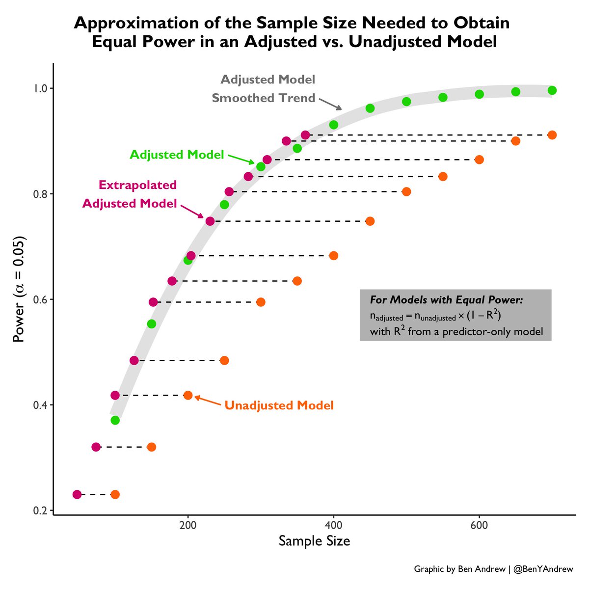
Here I simulated power for unadjusted & adjusted models in varying sample sizes, then used the conversion of n_unadjusted * (1 - R^2) to determine an extrapolated n_adjusted at the same power. The extrapolated n's line up nicely w/ the actual adjusted model sample size trend.

See @f2harrell's explanation:

https://twitter.com/f2harrell/status/1118481156037591042?s=20