Thread by @kdpsinghlab

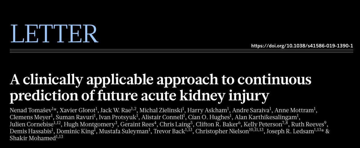
The DeepMind team (now “Google Health”) developed a model to “continuously predict” AKI within a 48-hr window with an AUC of 92% in a VA population, published in @nature.

Did DeepMind do the impossible? What can we learn from this? A step-by-step guide.

nature.com/articles/s4158…

To understand this work’s contribution, it’s first useful to know what was previously the state of art. I would point to two of @jaykoyner’s papers.

cjasn.asnjournals.org/content/11/11/… and
insights.ovid.com/crossref?an=00…

The 2016 @CJASN paper used logistic regression and 2018 paper used GBMs.

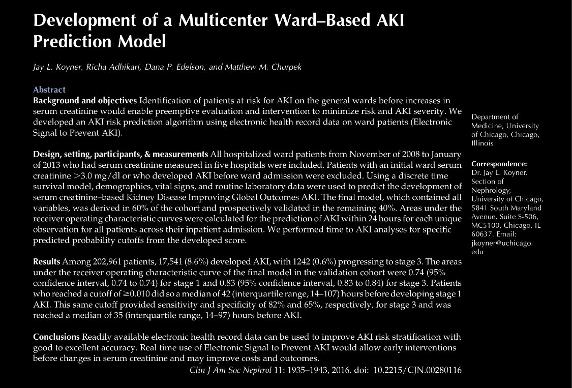
The 2016 CJASN paper is particularly relevant because it was also modeled on a national VA population. Altho the two papers used different modeling approaches, one key similarity is in how the data are prepared: using a discrete time survival method.

What the heck is that?

Discrete time survival is a method where time-to-event data is transformed by chopping it up into fixed intervals. So if a patient has no AKI at day 1 and 2 then AKI at day 3, this would constitute 3 data points if the interval is set to 1 day. Then you can analyze using logreg.

In Koyner 2016’s paper:
- selected interval wasn’t included in paper (“eg 12 hrs”)
- outcome window: 24 hrs
- lookback period was undefined
- missing values imputed by carrying forward
- Cr slope was included as predictor but no other slopes
- Cont variables modeled with splines

And the results in Koyner 2016 paper?

The best model had an AUC 0.74 for AKI stage 1, 0.76 for AKI stage 2, and 0.83 for AKI stage 3.

So the model is pretty good at detecting the “sickest” patients (AKI 3), right?

Not necessarily. AUC is the area under the curve that considers all values of true positive rate (sensitivity) and true negative rate (1-specificity). So in the setting of “class imbalance” where the outcome is rare, increased true negatives mathematically boost the AUC.

This, if AKI stage 3 is less common than AKI stage 1 or 2, then the rising AUC isn’t necessarily reassuring. From the main text of the Koyner 2016 paper, I can’t figure out the prevalence of each AKI stage — it may be in supp material or I missed it.

Let’s assume for the sake of argument that prior state of the art AUC is 0.83 across the board. Does machine learning get us much better performance?

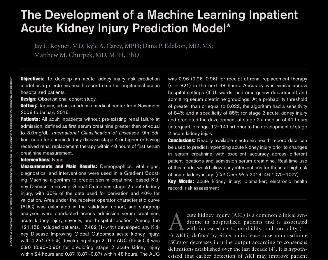
Koyner’s 2018 paper (on tertiary care center data) shows AUC 0.73 for all AKI and 0.93 for AKI stage 3. Performance better but..

...but the performance boost may not be entirely due to use of GBMs. A single center study (even if large) usually has more homogenous patients and data-generating systems (read: EHRs, order sets) so result in better models. But use of ML could be it, no?

This is where the @nature paper comes in. So without further ado, let’s jump to .... Supplementary Table 4?

Keeping in mind Koyner’s 2018 AUC of 0.73 for 48 hr AKI using GBM, the DeepMind team’s AUC for 48 hr AKI is....

... drumroll ... 0.89! Wait what? How is that possible?

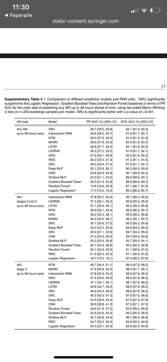
And logistic regression comes in at a horrific AUC of ... 0.86? Wow that’s pretty good.

So yes the headline is that an RNN achieved an AUC of 0.92, but the subheadline here is that other approaches (including the same GBM approach used in Koyner’s 2018 paper) got close. Why?

The magic (I think) is in the way the data is represented with a dash of help from the large sample size. The magic of RNNs added an AUC of 0.03 on top of GBMs (which the authors note is “statistically signficant”) but GBMs did well here. So did they use discrete time survival?

Although they never call it that, the DeepMind authors did something similar to the Koyner papers. They sliced data into 6 hour intervals then used prior 48 hrs of data (with optional longer lookbacks) to predict AKI in next 48 hours (actually next 72 but will focus on 48h only).

Key differences b/w DeepMind and Koyner 2018 papers in terms of data preprocessing:
- for each interval, many summary stats for each predictor were included (count, mean, median, sd, min, max)
- lagged and differenced predictors were included

In forecasting textbooks (plug for Hyndman’s book: otexts.com/fpp2/), lagged and differences predictors are key predictors. It’s not only impt what recent value of any lab is (a la discrete time survival). Older (lagged) values and how values are changing (diff) is key.

Once the data is represented in this way, it appears that the prediction task becomes a lot easier (and events per variable concerns are somewhat mitigated by the large sample size). Ok, now moving on to the headline: RNNs achieve an AUC of 0.92. Is this good?

Oooh just LOOK at that beautiful ROC curve. So far away from the dotted line (ok usually there’s a dotted line where y=x).

Don’t mind the SINGLE point from the GBM (which has a nearly identical AUC)... cough...

Ok so this plot provides no info, let’s move onto a plot that does.

This is the precision-recall curve. For the unitiated, precision = positive predictive value and recall = sensitivity. Remember how AUC ROC cares about true negatives? AUC PR doesn’t.

Left side of curve: capture all AKI by crying wolf

Rt side: be overly picky and capture no AKI

This plot is important for choosing a threshold. Altho dichotomization gets a lot of flak, it’s ok here because the way these early warning systems are typically implemented is by sending pages (or other interruptive alerts). So alert threshold needs to be determined.

For rare events, achieving a high precision (PPV) is hard. The authors decided that a PPV of 33% would be a noble goal (2 false alerts for every true alert).

At a PPV of 33%, the sensitivity was 35% at 48 hours. So they would miss 65% of cases, no?

The sensitivity of 35% is actually .. 55%?

I realize that the authors don’t use the term sensitivity directly but dang that is like the textbook description of sensitivity.

So what gives?

This is where things start to get messy. In early warning system lingo, I think of the terms lookback, intervals at which predictions are made, and outcome windows.

The RNN trained on a 48 hour outcome window but directly modeled 6 hour “steps” along the way.

So it turns out that the precision recall curve I was showing you was depicting the precision and recall for each 6 hour step and NOT for the 48 hour outcome window. You can see how step sensitivity is 35% for precision and only 55% when considering the full 48 hr outcome window.

I feel like this is a MAJOR miscommunication. The figure caption (2b) makes it seem like this precision-recall is considering the 48 hr look ahead whereas it is only considering the 6 hour step.

Does the AUC ROC suffer from the same interpretation issue? I can’t tell.

Here is why this matters. Prevalence of AKI will be a lot lower in 6 hr windows than 48 hr windows. Thus low AKI prevalence will inflate the number of true negatives and thus inflate the AUC. It’s hard to say whether this AUC is even directly comparable with Koyner’s.

It’s troubling that the authors cherry-pick the 48 hour outcome when it suits their preference (48h sensitivity of 55%) but define PPV based on the step only. The authors state this is because they are using the step to decide alert threshold but why not use 48 hr precision?

So let’s assume that the performance is indeed state of the art based on those caveats. The RNN approach appears to beat all other approaches. Why? What is an RNN?

Recurrent neural nets refer to a family a neural nets that model sequences of data (or non-sequence data that can be converted to sequences, eg images).

RNNs process data in batches and learn a state representation (coefficients) that serve as additional input to the next batch.

Recurrent layers can be stacked on top of one another, which broadens the flexibility that is being considered by the model. The coefficients (“weights”) and intercepts (“biases”) are learned via backpropagation. I won’t go in depth but will point out some cool things in paper:

When you backprop to fit model, you can simultaneously model multiple outcomes by including a loss function that averages error across outcomes. Simultaneously predicting lab abnormalities in the same model as AKI led to a 3% imp in AUC PR. Other papers have found this too...

So if you want to reproduce their analyses, ask the VA for the deidentified data they created AND SENT to DeepMind and then *checks code availability section of manuscript*, download Tensorflow.

Ok I think I’ll end there. Let’s discuss this paper. What did you find interesting?

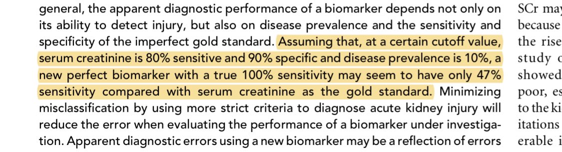
Ok the nephrologist in me would be sad to leave this out, and it is a point acknowledged by the authors:

Creatinine is an imperfect gold standard for AKI. It’s the standard of care at the moment but measurement error in the outcome is never a good thing.

ncbi.nlm.nih.gov/pmc/articles/P…

Also on a random note: in my son’s school, “begin with the end in mind” is one of the good habits he is being taught ...

... which is the same way I read this paper because somehow the methods section is AFTER the references? What kind of sorcery is this?

Clarification: true negative rate = specificity. AUC plots false positive rate on x axis, which is equal to 1-specificity. Since 1-specificity is on x axis, the AUC is the same as that if the x axis had been specificity (it’s the same area). Thus AUC is dependent on true neg rate